As sound reproduction has transitioned to the digital realm, audio professionals have a wealth of capabilities that were unthinkable in the analog days. Today, loudspeakers with companion digital processors are increasingly a tool of choice, going well beyond just the higher end of the application spectrum.

Virtually all types and brands of digital loudspeaker processors offer a rich suite of features, often overwhelmingly so. Some have capabilities that are unique, while others seek to capture the most important functions at the lowest possible price point. Nearly all provide a comprehensive set of functions that, if compared in a vacuum to the analog crossovers of yesteryear, would actually seem to be science fiction rather than reality.

The advanced capabilities—now often taken for granted—have unquestionably raised the performance potential of sound systems by at least an order of magnitude. But they also open a Pandora’s Box.

For example, how do we discern the choice of a Bessel curve over that of a Linkwitz-Riley? Why select a 12 dB/octave crossover slope instead of a 48 dB/octave slope? What’s actually going on with asymmetrical crossovers, extensive EQ capabilities, the use of digitally adjustable all-pass filters, incremental driver delay, phase filter controls, and the many other features that have become commonplace in the modern DSP loudspeaker controller?

Product user manuals do a great job of telling us how to access the various features of their products. But do we actually know why we might want to utilize these features? The answers are not simple and come from a deeper understanding of electro-acoustics, loudspeakers, and processing.

This is the first in a series of articles, to be continued regularly here on PSW in a step-by-step manner, to provide those answers. Here, we’ll start by looking at how to view and understand the on-axis and off-axis response of a typical single 2-way loudspeaker.

Importance Of Instrumentation
While many aspects of sound system calibration can be set by ear, it’s physiologically impossible to set up incremental time delays, all-pass filters, and phase filters relying solely on listening. Yes, you can select recommended crossover points and crossover rates, and even woofer delays from a loudspeaker manufacturer’s list of recommendations, and that might get you pretty far down the road.

But there is no substitution for taking the measurements yourself and making the optimal adjustments accordingly. Manufacturers are as overworked as the rest of us, and while most of them do their best to provide optimal guidelines, they don’t have access to all possible loudspeaker controllers, or in many cases, to optimal measurement instrumentation. For 17 years I was one of these folks. (By the very nature of the business, their suggestions are generic at best.)

Listening Vs Measuring
A common argument goes that “if whatever I do to adjust the equipment doesn’t sound better than before I adjusted it, then it’s meaningless.” On the surface, it’s a good argument, and it certainly applies to on-site, real-time mixing.

But dig one level deeper and you have to consider that whatever music you’re using as your guideline is written in a certain key and does not contain all possible fundamentals and harmonics.

For example, change the key from E to E-flat, and that nice, even bass line might suddenly reveal some holes or peaks in the response. Or, when the drummer shows up for sound check and re-tunes the kick drum to his preference, the tonality could change from tight and punchy to dull and mushy.

Moreover, trying to make micro-second alterations to mid-high crossover points – without the aid of instrumentation – is like trying to guess what bacteria looks like without using a microscope. It’s a sub-optimal condition at best. The only way to achieve the best possible result is through high-resolution measurement.

Let’s start with the basic process for optimizing a loudspeaker by looking at how to view the on-axis and off-axis response of a single 12-inch cone driver found in a typical 2-way biamplified loudspeaker.

Where pertinent, this will also include details on how the selection of each DSP signal conditioning choice was arrived at, and why each is important to the final result: making the loudspeaker as flat as possible within its operating range.

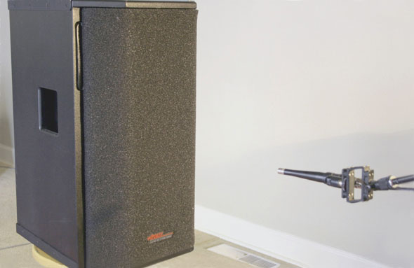
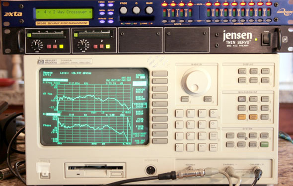
The measurements utilized for this article were conducted using a Hewlett-Packard 35665A dual channel FFT-based dynamic signal analyzer, a Jensen Twin-Servo 990 mic preamp, and a Bruel & Kjaer 4007 microphone. Equalization, where it appears, was performed with an XTA DP548 digital loudspeaker processor/controller.

All measurements were made in a near-field environment, within 1 meter of the loudspeaker, in a 45-foot and 25-foot carpeted room. The DUT (Device Under Test) was an Apogee AE-5 loudspeaker powered by a Hafler D-220 amplifier.

All signal level devices and the amplifier were tested with the HP analyzer to verify that they were flat within +/- .25 dB.

The B&K 4007 microphone was tested in relation to two other identical mics, none of which displayed a deviation greater than 0.5 dB from 25 Hz to 18 kHz.

Getting Prepared
Just as you’d advance an important gig, it’s important to “advance” your alignment work.

The loudspeaker you’re working with will probably be a commercial product, but maybe it’s home-grown.

Either way, information on the drivers should be readily available, and you’ll want that information close at hand. It might not bring you any great revelations, but it’s a starting point.

There are numerous high-resolution analyzers available these days that range in price from several hundreds of dollars that run on a laptop to many thousands of dollars for a sophisticated and dedicated highly engineered product.

Whether you spend a few hundred or many thousands of dollars, get your hands on one!

Let’s begin by looking at the response of the analyzer with the output connected directly to the input.

This is a simple exercise that I strongly encourage starting with, regardless of the analyzer being used, simply to establish a baseline that that verifies it is working properly and the cabling is correctly connected.

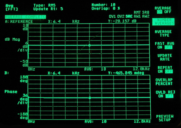
In the image above, the top graph shows frequency response from 0 Hz to 12.8 kHz, while the bottom graph shows the phase response in the same range. This is a linear frequency response graph, as it shows small variations that can be very important audibly, especially in the lower frequencies, as opposed to the more common log frequency graphs that tend to mask LF anomalies due to (usually) inherent lower LF resolution.

The graph stops at 12.8 kHz, merely to add greater clarity in the range of interest, but still depicts over 9 octaves of the 10-octave range of human hearing. Averaging was turned on only to make the camera shot clearer. In actual practice, the response is almost real-time with only 100 ms or so of delay between cause and effect. This response speed is precisely what you’ll want, especially when you’re moving your measurement mic from side to side and up and down to determine how a given speaker will respond off-axis.

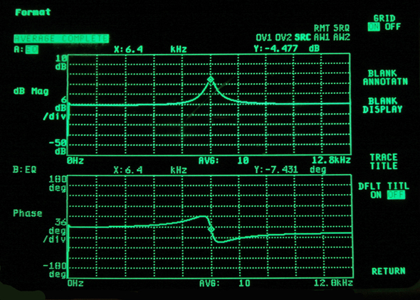
In this screen shot (directly above), we’re seeing the response of a simple peaking equalizer set to 6.4 kHz with an amplitude of about +14 dB (at this point, there is no loudspeaker in the measurement loop). The point here is to again verify that the measurement system is working properly and to show that for every IIR filter (Infinite Impulse Response), there is an equal effect in the phase response (see lower trace).

The phase angle will lead from the baseline before the peaking filter, than lag after it, but it will always be within a few degrees of zero at the exact center of the peak or dip of the IIR filter. This is an important step to understand by first developing experience with a stable source that involves no acoustical devices, before moving on to measuring transducers, and even more so, complex sound systems.

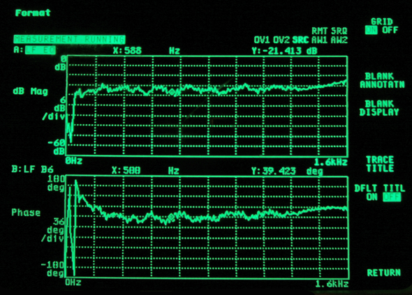
Now let’s look at an actual loudspeaker, a 12-inch cone driver in a well-constructed enclosure. The range is 0 to 1.6 kHz. No EQ or crossover of any kind has been applied. Notice that the frequency response is not very flat, but also not all that bad (incidentally, the measurement mic was about 0.5 meters from the driver). Also notice that the phase response is virtually the exact inverse of the frequency response, and also not so bad.

The big shift in phase response down around 60 Hz is the result of the phase inversion of the bass port (the test device is a ported enclosure). Phase inversion is a basic function of all ported loudspeakers and is not unique to this particular DUT (Device Under Test).

There are ways to compensate for the phase inversion, but they involve complex FIR filters and will add significant latency, and are rarely utilized. The practice is not common at this time in sound reinforcement, but is beginning to be seen in studio monitor systems where latency is not as critical as in live performance. (Just learn to get that punch-in button hit a little early!)

Here’s where it gets very interesting. This graph shows the exact same loudspeaker with the exact same measurement mic – in the exact same position – with five bands of EQ added to flatten the frequency response. You’ve probably been told throughout your career that EQ causes phase shift and too much EQ is something to be avoided. While EQ does cause phase shift, it’s not a bad thing if it’s correcting for anomalies that shouldn’t be there to begin with.

Look at how much flatter the frequency response is, as well as how much flatter the phase response is. In relation to the previous graphs, the phase response differential has been cut nearly in half, as has the frequency response differential. Both could be improved further by taking additional time to achieve more precision and by using more banks of the XTA DP548 equalizers.

So while it’s true that the application of EQ does indeed have an effect on phase response, it can’t automatically be characterized as a bad thing. Conversely, when executed properly, it’s a good thing as the graphs show. FFTs don’t lie.

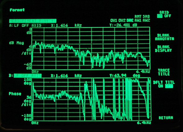
Now we’re looking at how the 12-inch cone driver behaves off-axis at about 30 degrees. Though this particular driver is perfectly capable of producing useful energy up into the 3 to 4 kHz range, that’s on-axis only. As soon as you get off the center axis, things start to fall apart, as will be depicted in the next graphic.

Notice how at 1.616 kHz (where the screen marker is located) the cone driver enters into its off-axis breakup mode and the response becomes highly irregular. By about 2,500 kHz, the phase and frequency response have become very poor. This is not something you want your off-axis audience members to hear. Understanding these parameters can make a huge difference in how you choose to adjust your DSP crossover settings.