A listener at a distance remote from the loudspeaker will pay more attention to the direct field of the loudspeaker than sound that is building-up in the room. A microphone gives equal weight to all energy without regard to where it is coming from.
A simple experiment to verify this is to stand at the microphone position and listen to the loudspeaker and then route the mic through a headphone amplifier and listen to it through headphones – not the same thing at all.
Low frequency sounds tend to linger in rooms longer than high frequency sounds, because most rooms have more high frequency absorption than low frequency absorption.
As such, the room becomes “bass heavy” when the total sound field is considered. This extra low frequency information will dominate what is observed on the RTA, and the knee-jerk reaction is to attempt to “flatten” the response by boosting the high frequency bands on the equalizer.
The result is a system with excessive high frequency output and a resultant “harsh” sound quality.
When RTAs are used in this manner, it is important to equalize to a “target curve” rather than for a flat frequency response. The popular “X” curve for theaters is flat to 2 kHz, where it starts rolling off the high frequency response at about 3 dB per octave. It is -10 dB at 10 kHz relative to 2 kHz.
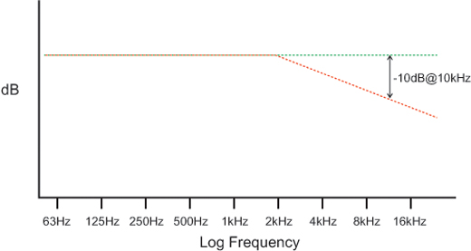
This represents 1/10th power at 10 kHz relative to flat response. The one-third-octave analyzer and the target curve have served sound practitioners well for years, and remains a viable approach to system calibration.
Recent Methodologies
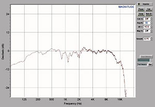
Technology has yielded some new methods for acquiring the system response at a listener position. A complex comparison (both time and frequency information) of the input and output of a system is called the transfer function. It includes both the magnitude and phase response of the loudspeaker/room at the microphone position.
This has become a popular method of analysis, as it allows any input stimulus to be used to test the system, since the displayed response is just the difference between “what you put in” and “what you got out.”
Transfer function analysis has the added advantage of the ability to use a “time window” to exclude late arriving energy from consideration in the response. This can prevent the low-frequency build-up problem that plagues traditional real-time analysis. With proper implementation of a time window, the system response can be adjusted without the need for frequency weighting via a target curve.
A major difference between transfer function analysis and 1/n-octave real-time analysis is that the former requires the removal of the signal delay between the two signals being compared. The stimulus (the reference signal) always has a much shorter path back to analyzer input than the output of the measurement microphone. Sources of delay include the travel time through the air and the latency of digital processors.
Failure to properly synchronize the reference signal and the microphone’s signal will result in an erroneous display of the system’s response. The length of the time window must also be selected – in other words, “how much of the room decay do I want to include in the response?”
Unfortunately, there is not an optimum size for the entire spectrum. A short time window excludes much of the room decay at the expense of low-frequency resolution. A long time window improves frequency resolution at the expense of gathering too much of the room’s decay. A compromise is required.
The human auditory system perceives pitch on a proportional (logarithmic) frequency scale. This is one reason that we use constant-percentage bandwidth filters for tuning audio systems – the bandwidth grows with increasing frequency.
Frequency-dependent bandwidth suggests that the length of the windowing function used in transfer function analysis should be varied in the same manner—a decreasing length with increasing frequency. This produces a somewhat “anechoic” response at high frequencies with increasing frequency resolution as frequency decreases.