
Author’s Note: Following its original publication [1] in May of 2021, I was notified of an error in tabulation regarding the data in Figure 12. This second edition provides the corrected values in Figure 3, below. Also, five new sections have been added or updated: The Wave/Ray Duality of Sound; two real-world reports on T60 Slope Ratio (TSR) and Parametric Method of Acoustic Treatment (PMAT) applications at work; and commentary on the ideal T60 and variable acoustics. In addition, several sections have been rewritten to provide better clarity.
The topic of architectural acoustics has been documented and carefully studied for more than a century. Historically, most acoustic treatment products and schemes have offered a relatively “broadband” approach to managing reverberation in a room. While this fundamental approach has changed little, acoustical goals, priorities, training, and materials need updating; each needs to incorporate and correlate a broader range of frequencies, while addressing their unique, quantitative relationship to one and other.
Why? Because of the massive amounts of full-bandwidth energy being pumped into rooms deploying our modern loudspeaker technologies.
The Parametric Acoustics thesis does not challenge the physics underlying traditional acoustic theory. Rather, it offers a fresh perspective on how new materials can and should be deployed.
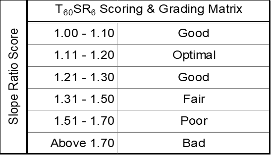
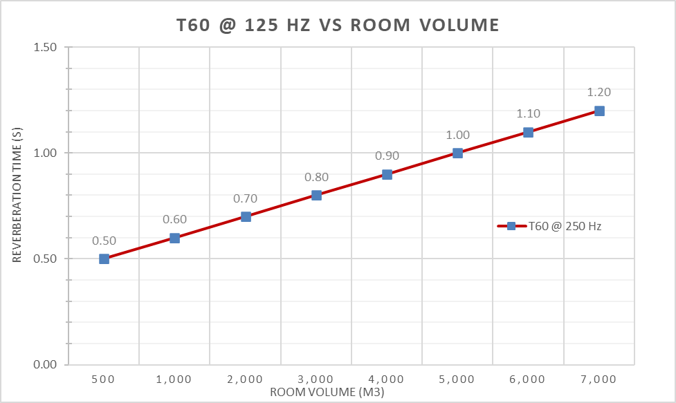
This paper expands the T60 Slope Ratio thesis [2] by providing methodology, commentary, and examples for specifying acoustic treatments as band-limited tools. The T60 Slope Ratio (TSR) is represented symbolically as T60SR6. The calculation delivers a relational score (Figure 1) using the two extreme time values — from the six octave centers — between 63 Hz and 2 kHz. The score is calculated by dividing the longest T60 by the shortest T60, regardless of octave.
This discourse outlines how a “Good” to “Optimum” TSR score can be achieved in any performance venue. To that end, the next level of architectural acoustic refinement is proposed: PMAT — the Parametric Method of Acoustic Treatment.
While the best practitioner’s in architectural acoustics already understand, and may implement similar principles, the PMAT concepts are not widely considered or applied.
Background
Professional-grade loudspeakers are designed and optimized to perform as flat, or nearly flat (magnitude), audio output devices. Therefore, shouldn’t acousticians be designing the same nearly-flat timbre into the rooms in which these loudspeakers operate?
TSR theory prescribes a set of design and performance goals that encourage us to craft a nearly flat reverberant room response, but doesn’t offer any specific treatment guidelines to achieve those goals. PMAT adds methodology to this new model of refinement in architectural acoustics.
The idea of a generalized, single number reverberation time is merely a convenient way of stating a room’s averaged mid-band (500 Hz and 1 kHz) reverberation time (T60 or T30). For most end users, acoustics boils down to this single-number concept. It’s not uncommon to hear someone say, “We have way too much reverb in this room for the style of music we’re trying to present. It seems like it lasts about two seconds.” Knowingly or not, this commentary is almost always referring to the mid-band reverb time (Tmid) in their room.
Unfortunately, these remarks often lead to the ubiquitous, 1- or 2-inch, fabric-wrapped fiberglass panels, or similar foam products. If all you need to do is reduce reverberation at 500 Hz and above, these products may be all that’s required.
Notice the common theme with each of the products shown in Figure 2: very low absorption coefficient (α or alpha) values at 250 Hz and below, then a quick rise to much more useful numbers, starting at roughly 500 Hz.

The various T60 charts shown below have an inverse slope or shape to those of these popular treatment products. Essentially, these materials perform as 500 Hz, low-pass, reverberation and resonance filters. Or, exactly the opposite of what a room might need most.
Absorption Coefficients Above 1.0
The sound absorption coefficient is the fraction of sound energy absorbed by a material. Expressed as a value between 1.0 = perfect absorption (no reflection), and 0 = zero absorption (total reflection). The value varies with frequency and angle of incidence, determined experimentally. [3]
If you’re disturbed by the various charts in this document showing alphas higher than 1.0, know that I am aware of the arguments for, and against. The data used herein comes from the various manufacturers cited. If preferred, round down to 1.0. By lowering to a max α of 1.0, your results will merely reflect the need for more material.
PMAT Defined
PMAT theory suggests that acousticians specify products and materials that not only perform broadband absorption when required, but also perform specific work within various 1- to 2-octave bands. Think of these products as 1- to 2-octave, cut only, parametric absorbers (room-tone equalizers).
An electronic, parametric equalizer offers separate controls for frequency, bandwidth (Q), and level. When properly applied, these are powerful tools. If we adapt those same three parameters to material alphas, we introduce a completely fresh, band-specific way of treating excess reverberation and resonance.
- Frequency: The center frequency of maximum absorption offered by the treatment material.
- Bandwidth: How broad or narrow is the Q? PMAT theory suggests that when the α rate is reduced by 25% or more – one octave above and below its peak α – and continues to fall off on a similar trajectory, then the product may be well-suited for PMAT applications.
- Level: Higher alphas are better. The higher the α, the more effective the product is at absorbing energy at that specific frequency. This translates to less material being needed per frequency band, and lower overall cost.
Line Charts
Using line charts [4] is probably the easiest way to visualize and understand reverberation time at the various frequencies of interest. They’re also good for showing alpha data.
Many of the line charts presented in this thesis use the standardized, one-octave frequency centers, between 63 Hz and 4 kHz. While excess 4 kHz reverberation is rarely an issue, it’s shown because most of the manufacturer’s spec sheets extend the range of their α data to that frequency. 1/3-octave bands can and should be used if a room exhibits an unusually-strong or asymmetrical distribution of resonance or reverb between the octave centers.
Describing how to gather the necessary acoustic data is outside the scope of this paper, but know that modern FFT measurement platforms (i.e., Rational Acoustics Smaart and AFMG SysTune) capture impulse response data that can be analyzed at both octave and 1/3-octave resolution.
What’s So Special About The “Slope”?
In a well-behaved room, regardless of its Tmid time, the incline or slope of its T60 line chart will gradually decrease, beginning with the lowest frequency analyzed. This is a natural and expected profile, primarily controlled by a combination of room size and geometry, finish materials, and air absorption. For rooms equipped with powerful, full-range sound systems, TSR theory suggests the slope should be nearly flat – with only a very gentle, downward tilt – from 63 Hz to 2 kHz.
Beyond simply containing excess low- (LF) and very low-frequency (VLF) reverb and resonance, when a room presents an “asymmetrical” or “double knee” slope (see the broad red line chart at the top of Figure 12), any of the six octaves may contain a much longer or shorter reverb time than its neighbor. When looking at a well-contained T60 chart (see the broad green line chart in Figure 12) there should be no sharp knees. Ideally, those anomalies can and will be addressed using PMAT solutions.
Needs Analysis
Every room or building has some inherent acoustic “sound” or tonal character. A few are complementary to their various sound-related functions, others are obviously bad – even to the sensitivities of the non-professional. The vast majority fall somewhere in between, and do not fully reveal their strengths or weaknesses until certain sonic activities are introduced.
The exceptional rooms generally go unnoticed to all but a few, whereas really bad rooms seem problematic to almost everyone; usually because they have too much reverberation for almost any application.
One bad example is a high school gymnasium I reviewed many years ago. There was so much reverb the coaches couldn’t hold basketball or volleyball games, or practices. They couldn’t communicate with the players. The %ALcons score was 33, which translates to an STI score of 0.30; both are considered “poor” results.
For this building the obvious solution was lots of broadband absorption. Because this wasn’t a performance venue, and didn’t require custom or specialized treatment, the solution was the application of about 9,000 ft2 of International Cellulose K13, sprayed on the ceiling – to a thickness of 1.5 inches.
While this was an extreme example, most venues have more specific needs. If we’re within about one second of an appropriate Tmid time it is suggested here that alone, broadband absorption is not the only, or best answer.
As stated earlier, most broadband treatment materials, like those shown in Figure 2, provide inadequate absorption at or below 250 Hz. This is a problem because these days many performance, worship, and entertainment venues can’t dissipate the massive amounts of LF and VLF energy as quickly as it’s being produced by the loudspeakers.
To further complicate matters, it’s also likely that the 63 Hz and 125 Hz octaves aren’t the only ones with resonance or reverberation that’s too long – relative to their neighboring frequencies. When such scenarios exist a room’s reverberant character is even more out of balance and should be “acoustically equalized”.
For example, consider the survey done by Dr. Niels Adelman-Larsen (NAL) in his book Rock and Pop Venues – Acoustics and Architectural Design. [6] Figure 3 represents an aggregate of the 10 best and worst venues for Rock and Pop music in Denmark.

Pay close attention to the T30s at 63 and 125 Hz in these 20 venues. The Tmid average for the “Best” rooms is 0.87 seconds, and for the “Worst” rooms it’s only 1.05 seconds. The point: One would think a 1.05 second room should work well for amplified rock and pop music. However, acoustic problems often lie well below the Tmid bands. They lurk in the bottom two or three octaves. This is where these rooms have trouble dissipating the constant flood of LF and VLF energy.
Even the chart labeled Best, represents a T60SR6 score of 1.37, which translates to a “Fair” MOS (mean opinion score) grade. For the Worst venues, the average score is 1.43, which also gets a Fair grade, but it’s a mere 0.07 seconds away from being considered poor; before the audience arrives.
Like most reverberation measurements, these times were captured in unoccupied rooms. “The data shows that the absorption coefficients of a standing audience is five to six times higher in the mid-high frequency bands, and that there is very little absorption in the low frequencies”. [5a]
The take away is this: A room that has a “Fair” TSR grade when empty, can easily turn into a “Poor” room when occupied. Therefore, it’s important to start with the best possible TSR score so when the room is fully occupied, the slope ratio is less impacted for the worse.
While twenty venues is a relatively small sample size, the trend is obvious: none of these rooms were designed with our modern musical tastes and technologies in mind.
Is There An Ideal T60?
There is no ideal T60. The best we can offer, based on static rooms without variable acoustics (VA), are suggestions based on the music genre and the volume (size) of the room.
For example: Figure 4 briefly summarizes the results of the research [5b, 6] done by NAL, which concludes there are two important factors to consider for rhythmic music genres (i.e., rock, pop, jazz, punk, hip-hop, Latin, and contemporary worship, etc.): room volume and T60 at 125 Hz.
These two quantifiers have been distilled from RIR (room impulse response) measurements taken in 20 small to mid-sized halls, and 33 engineer/musician surveys [5c, 6] NAL conducted in Denmark. They conclude that – depending on room size – a wide variety of rhythmic music genres sound best when performed in rooms with about one-half second to one and one-quarter seconds of reverberation/resonance at 125 Hz. His various publications [5a, b, c] place a great deal of emphasis on these two fundamental values.
The Wave/Ray Duality Of Sound
Sound behaves differently depending on wavelength (frequency) and the environment in which it is propagated. Dr. Manfred Schroeder referred to the frequency at which rooms go from being resonators to being reflectors/diffusors as the “crossover frequency.” We now call it the Schroeder frequency (FS). [7]
The formula for determining the Schroeder Frequency is:
Where T30 is the Tmid reverb time, V is the room volume in feet or meters, and K is the constant. K = 11,885 (US) or 2,000 (SI). The environment mentioned above is an enclosed room, regardless of size. Together, room volume and its Tmid reverberation time determine the FS point.
FS defines the initial (lowest) frequency, beyond which all lower sounds behave like waves. Once you know FS it’s necessary to multiply that frequency by four (4) to determine the upper limit of the “transition zone” (4FS). 4FS establishes the point at which all higher sounds behave like light rays.
The transition zone consists of frequencies with ambiguous behaviour; neither fully resonant/modal, nor completely diffuse reverberation. This is not a hard transition but a gradual one, which occupies about two octaves of sound, and includes all frequencies between FS and 4FS.
Application: If FS is 70 Hz, then T60/30 measurements of a room are only reliable above 280 Hz. It takes a very large room – over one million ft3 – to reliably evaluate true reverberation at, or near, 63 Hz. In other words, just because you have excess reflected energy in a room at 63 Hz, or 100 Hz, doesn’t mean that the energy is reverberation. More likely it’s modal resonance.
Note: There is no such thing as a “ray” or “particle” of sound. The ray descriptor is used just for simulations. All sound travels in waves. Room modes don’t stop at FS or 4FS, they extend over the entire audible spectrum. At and above FS the mode density is so high that the modal math becomes impossibly complex. So, to simplify things, we transition to geometric acoustics based on optical principles. If we have accurate input data, and could crunch the numbers, our predictions would use the wave equation for the entire audible spectrum.
In his recent article [8] on the Schroeder Frequency, Pat Brown calls the transition area between Fs and 4Fs the “diffusion zone.” These are the frequencies that behave a little like both waves and rays.
Generally, reverberation produces the same diffused sound levels for all listeners. It has no specific direction of energy flow.
On the other hand, room modes (standing waves or eigentones) produce dramatic level changes from location to location – often separated by only a few feet. Figure 5 is a great visual. It tells the story better than a thousand more words could. It also helps explain why one person will complain that the bass is overwhelmingly loud, while someone sitting just a few feet away may observe that there is not nearly enough.

Why is the wave/ray duality relevant to PMAT? For truly effective results, acoustic materials need to be selected based on the frequencies needing treatment. “Modal zone resonance (at and below FS) requires active trapping such as found in diaphragmatic panels, bass traps, and Helmholtz resonators. Diffusion zone frequencies (FS to 4FS) often respond best to physical objects such as wall shape, furniture, and complex surface finishes with deep relief. Only at, or above 4FS, can we expect adequate performance from the “typical” acoustic treatment materials such as carpet, padded chairs/pews, fiberglass wall panels, and people.” [8]
Even though room modes aren’t technically reverberation, the fact that they exist, and may resonate longer than all other low-, mid-, and high-frequency reverberation, means they still can muddy-up a mix, and must be treated in order to improve the “music clarity” of a sound-reinforced performance.
Pay Close Attention To Absorption Coefficient Specs
The α values of any treatment solution should have a certified laboratory report that can be easily accessed from the manufacturer’s website. The basic assumption is the data follows standardized ISO or ASTM testing procedures.
First caution: When evaluating treatment materials, check whether metric or imperial sabins are being stated. The sabin is the unit of measurement used to describe a unit of sound absorption. “One square meter of 100% sound absorbing material has a value of 1 metric sabin. One square foot of 100% sound absorbing material has a value of 1 imperial sabin.” [3] The obvious conflict is: it takes 10.76 square feet of material to equal 1 square meter of the same material, so it’s easy to make a huge mistake if you don’t know which one you’re working with.
Second caution: Beware that some manufacturers state the absorption data per square foot (or meter) of exposed surface material on some items, while for other products they report the data for the unit as a whole. If the data is clearly marked as representing a “per panel” or “per device” value, it’s fairly easy to calculate back to a value that represents the α per square foot or meter. Example: A 2’ x 4’ panel has 8 ft2 of surface on one side. Divide the per-panel sabins total by 8 to get the α per square foot.
One way to spot the difference is to watch for alphas that are well above 1.0, and often above 2.0. If you see this, there’s a good chance the data is being expressed for a whole panel.
Current High Q Products
Wouldn’t it be great if there were lots of treatment options based on selective, octave-band absorption? And, wouldn’t it also be cool if those options included both velocity- and pressure-based absorption schemes? If you’re unfamiliar with the differences between velocity- and pressure-based absorption, this short article [11] from GIK Acoustics is quite concise.
Finding existing products to fit the specific needs of a project can be difficult. I’ve spent considerable time looking, and will share several examples below. Hopefully, in the near future, more manufacturers will see the value in developing band-limited absorption products.
When considering bass-range treatments, it’s important to determine how a manufacturer’s absorption data was tested. Some companies provide their α data based on impedance tube measurements, which only give normal incidence alphas. A very large reverberation chamber is needed to accurately measure random incidence sound absorption coefficients.
Notice the similarity between the shape of the T60 line charts and the alphas of the potential treatment solutions highlighted below. This is what we’re looking for from all potential PMAT products. The longer the T60 at any given octave center, the greater the alpha we want at that same octave center.
Remember, it’s necessary to view the charts below as inverted, parametric cut filters. In other words, the higher the peak α, the deeper the acoustical cut.
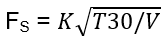
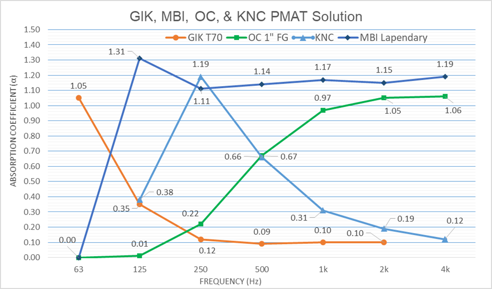
Both RPG and GIK Acoustics show dedicated “bass trap” products that represent what we’re looking for at 100 Hz and below. Check out the α chart for the GIK Scopus series and the RPG Modex Corner series bass traps (Figures 6 & 7). These examples show significantly lower alphas above and below their peak absorption frequency.
Note: At publication time I was introduced to RealAcoustix, which offers multiple bass trap options that have been tested in the large chamber at NWAA Labs in Washington. [12]


Figure 8 shows some excellent examples at 125 Hz, 250 Hz, and 500 Hz.
The RPG Modex LF product has a very nice α chart that peaks at 125 Hz. The Kinetics Noise Control (KNC) — Sereno 2/10 2” FG – perforated wood panel fits nicely into the PMAT scheme. Notice how quickly it falls to 0.38 at 125 Hz and 0.66 at 500 Hz. Also, you can see how this panel is used to address the 250 Hz slope asymmetry in Figs 11 & 12 below.
At 500 Hz – the best example I’ve found is the MBI 2” Bandit series. It has a slightly broader Q at 1 kHz, but overall it fits well into the portfolio.
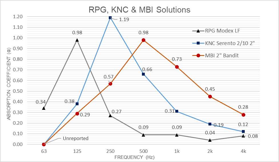
Figure 9 shows another interesting 125 Hz product. The Mega Trap, from Real Traps, boasts 2.66 sabins of absorption, per ft2, at 125 Hz.
Figure 10 takes us up to 1 kHz: The 1.2-inch RPG BAD Panel actually peaks slightly lower at 800 Hz, but it’s the closest option found for addressing 1 kHz. It’s really best applied when a little broader PMAT solution is needed.

I have yet to find anything that specifically addresses 2 kHz and above, but alone those frequencies are rarely a major concern.
By now you should begin to see how the PMAT theory is applied. As always, the application of these treatments needs to be well distributed and properly positioned to maximize their effectiveness.
Adding Sabins From Different Materials
How do the various α values add together, at any given frequency, when working with materials having disparate alphas? The answer is to convert the various alphas into total sabins of absorption at each frequency of concern.
Let’s say you have 128 ft2 of a treatment that has an absorption coefficient of 0.60 at 500 Hz, and 128 ft2 of another product that has an α of 0.35 at the same frequency. You don’t get to add the alphas together. Based on area, you have to calculate the total sabins of each, then add those numbers together. Example: 128*0.60 = 76.8 sabins of absorption from material A, and 128*0.35 = 44.8 sabins from material B. Together, these add up to a total of 121.6 sabins of absorption at 500 Hz.
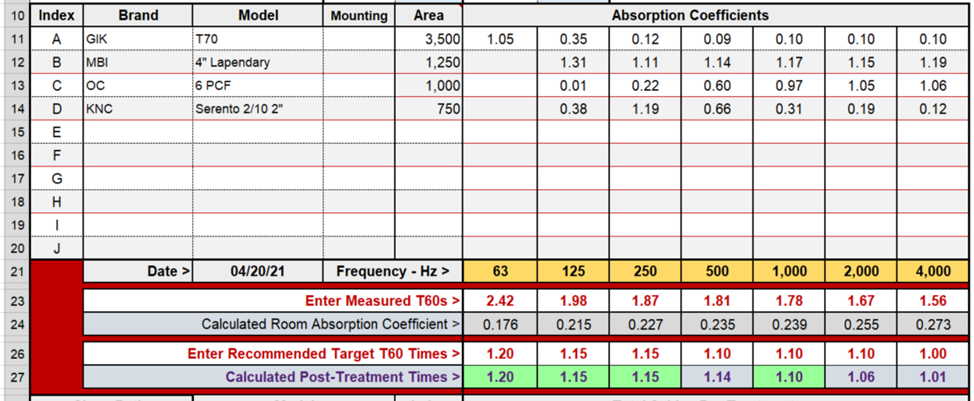
To help organize and crunch these numbers, I’ve created a Rough Order of Magnitude (ROM) sabins calculator. (Figure 11) This is a statistical calculator that requires T60 data from an existing (or modeled) room if you want to calculate before and after treatment results. For budgetary planning, it’s a reasonably objective way to estimate the approximate square footage of each material needed to achieve your new T60 goals.
The measured T60 data establishes the existing conditions in a room. The existing conditions are described as “Room Absorption.” Per IEC 801-31-11, Room Absorption (RA) is the sum of sabin absorption due to objects and surfaces in a room, and due to dissipation of sound energy in the medium (air) within the room.” [3]
To calculate the existing RA for each frequency, the known T60 times are input along row 23. The absorption coefficients will be automatically calculated along row 24 — using Sabine’s classical formula.
Column F, from Rows 11-20, is used to input and manipulate the total area needed for each treatment material considered. Target T60 times are input along Row 26. The underlying formulas in Row 27 calculate the effects of the various treatment alphas, based on the total square footage of each material applied at each frequency. The cells in row 27 turn green when you’ve found an exact match.
It’s not necessary to perfectly match the times in rows 26 and 27, but they should come close. Try to stay within +/- 0.10 of a second. 4 kHz may be the hardest to match, but it’s the most forgiving, so +/- 0.15 seconds or so should be close enough.
The Figure 12 line chart displays all the key values shown in Figure 11, including the asymmetrical T60s of this hypothetical, untreated room; the room’s estimated post-treatment T60; and the absorption coefficients for each of the materials selected to reach the target goals.
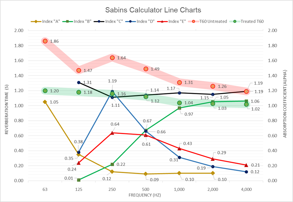
Remember: This is a ROM estimator. It’s impossible to calculate and predict perfect results. This spreadsheet is simply a tool to help organize the data and streamline the numerous calculations, which are tedious to process.
This sabins calculator can be downloaded [9] from the GraceNote Design Studio website. V2.2 now includes a Schroeder Frequency calculation block in the lower left corner.
More Examples with Varying T60 Profiles
Over the past thirty years or so we’ve seen house of worship music shift fairly radically: from the traditional/classical genre with mostly acoustic instrumentation, to today’s worship music that’s contemporary, rhythmic, and often quite loud. However, in many instances, the acoustic environments have not been adjusted accordingly, if at all.
Below are three more examples of how PMAT solutions might be, or have been applied. The first (Figure 13) represents a hypothetical, highly reverberant church sanctuary with a 1.80 second Tmid – which rises to 2.42 seconds at 63 Hz. Untreated, this example gets a “Fair” grade based on a T60SR6 score of 1.45. A venue such as this may have been wonderful for mass choir, pipe organ, and/or orchestra, but it’s not acoustically “friendly” for modern-day amplified music, nor spoken word intelligibility.
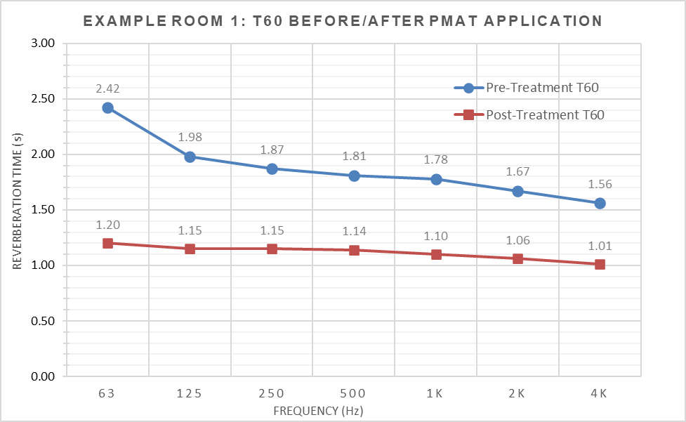
Suppose this hypothetical church wants to modernize their worship music programming. What will their acoustic challenges be? It isn’t too difficult to reduce the overall mid- and high-frequency T60s, but to bring the TSR up to at least a “Good” grade, the 63 Hz and 125 Hz octaves must also be addressed.
Currently, no known single product can address every adjustment that may be appropriate for this example. As many as four PMAT filters may be needed.
Hypothetical Example Room 1
Because it will drive all other acoustical decisions, setting the various new goals should begin with the Tmid conversation. If, because of genre or budget, the goals need to change to either a longer or shorter Tmid, only the quantity of each material needs adjusting.
For this 177,000 ft3 (≈ 5,000 m3) room the basic post-treatment metrics of concern are as follows: Tmid target – 1.10 seconds; 125 Hz T60 target – 1.15 seconds; and an Optimal TSR grade. Figures 14 and 15 below show examples of how this PMAT solution was calculated.
We now have the guidelines and tools needed to estimate and specify appropriate materials for a room like this. Of course, the placement of each material requires careful analysis and execution, as well as customer approval.
Hopefully, the way all these metrics work together is beginning to make sense. They attempt to define, shape, and deliver the best possible acoustical characteristics in a room.
Example Room 2 – 25 Year Old Presbyterian Church
Example Room 2 (Figures 16 and 17) is a work in progress. This example is based on an architecturally-challenging, 99,100 ft3 (≈ 2,800 m3) sanctuary, located near Irvine, CA.
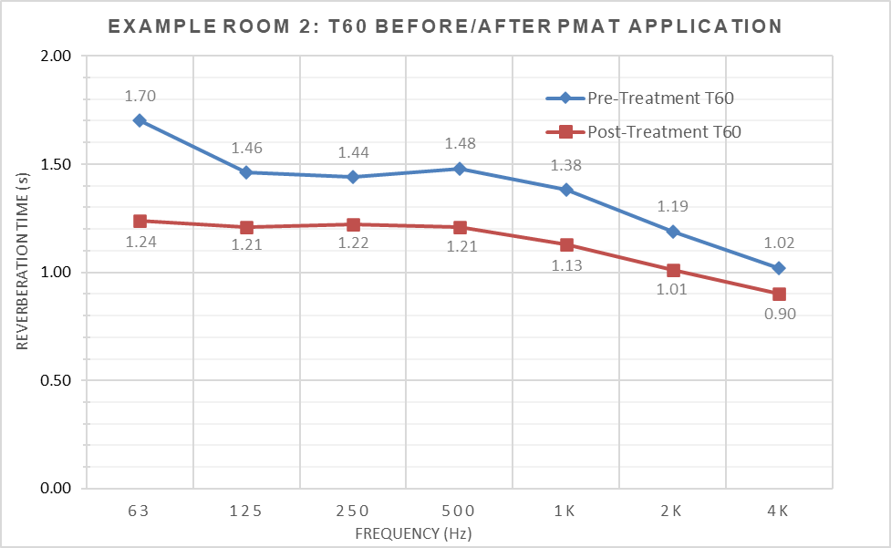

Final test results will not be available anytime soon, so only estimated results are shown. The results are based on the recommended solutions, which were plugged into the sabins calculator. In other words, this is a real world example of how PMAT works in the planning stages of a project.
The church has modernized their worship music, which is now “light” contemporary. Acoustically, their main complaint is “boomy and muddy sound”. These comments aren’t too hard to imagine after looking at the “before” RIR measurements. The room’s initial Tmid is 1.43 seconds. The current TSR grade is Fair.
Moving forward, the goal is to lower and smooth out the room’s reverb and resonance profile so it falls within, at least, the Good TSR range. The new Tmid target is 1.25 seconds, or slightly less. Based on the “after” treatment predictions, those goals should be achievable.
The treatment solutions shown in Figure 17 consist of: 200 ft2 of the Mega Trap product, 850 ft2 of the Modex Corner 62 product, 100 ft2 of 2” Bandit product, and 500 ft2 of fabric-wrapped, 1-inch fiberglass paneling.
Interesting note: As mentioned earlier, the architectural structure of this room is very challenging. It has a fan-shaped pew seating footprint (with curved pews), which is placed in a + (plus) shaped structure, with radically-varying, non-symmetrical ceiling heights.
Ordinarily, the 1-inch fiberglass paneling would not be specified for this project because it does too much work between 1k and 4k. But, because of the awkward (and only reasonable option) point-source loudspeaker positions, something has to be installed to minimize the slap echo off the hard, parallel, vaulted-ceiling surfaces that the loudspeakers fire under (long story). Diffusion panels would be a better option, but cost, aesthetics and weight considerations rule out that preference.
Example Room 3 – Saddleback Church
Saddleback Church, in Lake Forrest, CA, serves as a real-world example of the applied PMAT process. Because of their loud, contemporary worship style, the church representatives expressed a specific appeal to not only reduce the overall reverberation in their worship center, but also include a custom solution to address the excess LF and VLF resonance and reverb.
The Saddleback Worship Center is quite large, seating just under 3,000. The room is roughly 1,084,500 ft3 (≈31,000 m3), with lots of highly-reflective glass and steel. The Schroeder frequency is 17 Hz. When the 4FS multiple is applied, it shows that the room is sufficiently large to develop true reverberation down to 68 Hz. This means everything that sounds like reverb, below 68 Hz, is most likely modal resonance.
To reduce the overall Tmid by about 1 second, it took a little more than 12,000 ft2 of hanging 2” fiberglass (6 PCF) baffles; over 7,000 ft2 of hanging 2-inch cotton (3 PCF) baffles; about 2,700 ft2 of R-30 batt insulation; and 20 huge, custom-tuned bass trap resonators.
While the majority of the absorption work was accomplished with these products, a new line array system — with cardioid subs — also helped reduce the indirect energy being pumped into the room.
Finding appropriate locations to install all these treatments was challenging. Attachment to the walls was not allowed. The single largest area available was the ceiling. There, edge-hung baffles could be installed just below the corrugated-steel roof deck, delivering 64 ft2 of absorption from each 4’x8′ panel. A case study report on this project can be found here: [10]
There’s little doubt that the 2-inch baffles helped somewhat at 63 Hz and 125 Hz, but all those 6 PCF baffles have the same absorption profile as the 2-inch Owens Corning panels shown in Figure 2. Figure 18 reveals that, by themselves, the hanging panels would not provide all the LF and VLF control that was desired.
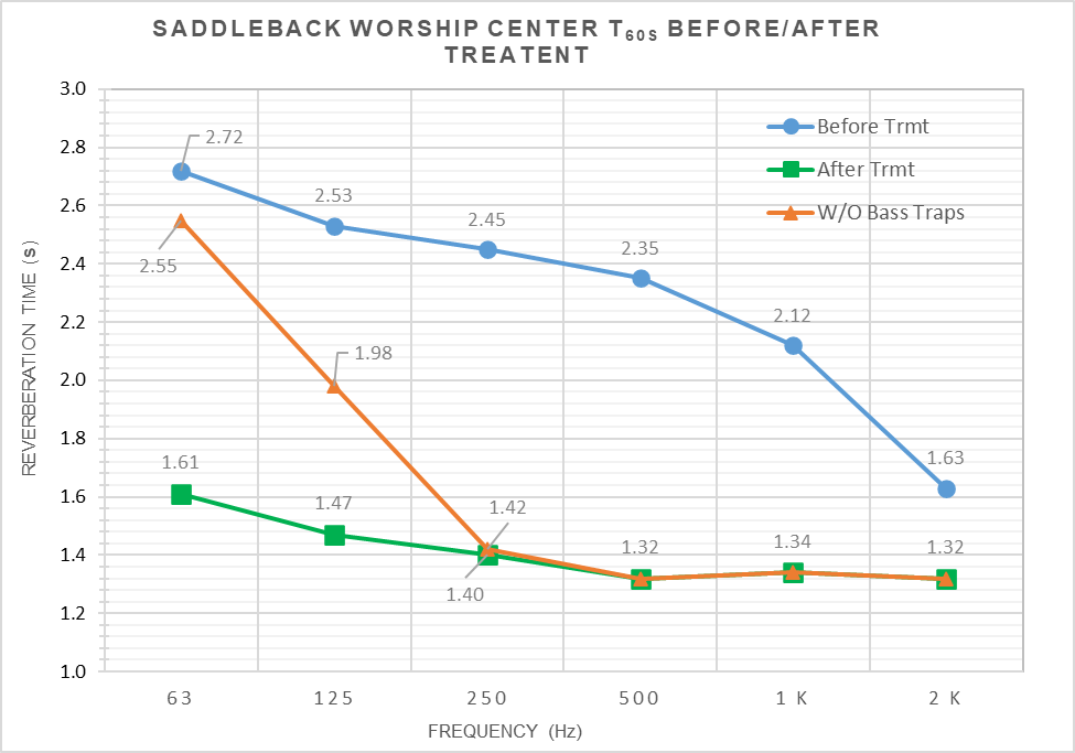
Here’s an example of how location and mounting techniques can make a tangible difference: There was a large area where LF and VLF energy would build up below the retractable stadium seating at the back of the room. This is where the majority of the cotton baffles were hung; soaking up much of the unwanted low-end reverb and resonance where it developed.
Pivotal elements that influenced winning the contract for this project were the clear understanding of the customer’s overall acoustic problems, the proactive design processes used to address their structural and aesthetic limitations, and a commitment to resolve most of their low-frequency challenges.
What About Variable Acoustics?
Is all this necessary if you have, or are planning for variable acoustics? The short answer is: probably. Some electro-acoustically controlled VA schemes are additive — adding reverb to a room that’s too dry. Examples are the Meyer Sound Constellation, the E-Coustic Systems Gen 3, and the Muller BBM Vivace.
Some are subtractive – absorbing, or cancelling, reverb and resonance. Examples are the Flex Acoustics Evoke and aQflex systems, or the Bag End E-trap. A third variation comes in the form of manual systems that require opening and closing drapes, rotating adjustable panels, or opening/closing secondary reverberant chambers.
Deploying a VA system is pretty much a one-way street; you can either add or subtract reverberant energy. But, you can’t subtract energy using an additive system, nor add energy using a subtractive system. Each scheme has limits to what can and can’t be controlled. Therefore, the primary question becomes: What does the room’s tonal character (its Tmid and TSR grade) need to be before any VA scheme is installed?
Final Thoughts
When my career in pro audio and acoustics began I never expected to find myself so focused on the nuances of large room reverberation. Over the years, a prime tenet has been to look for the weakest links in my audio and acoustic toolboxes, then work to strengthen those weak links as much as possible. To that end, I’ve long believed the weakest link in architectural acoustics is the lack of interest and attention paid, by most practitioners, to identify and treat resonant and reverberant energy – at and below 125 Hz. Most of the acoustic material manufacturers are guilty as well.
For venues offering 21st century amplified music and production, acoustic standards and specifications should target appropriate Tmid and 125 Hz goals, while also applying customized PMAT solutions to achieve the best possible TSR score; thereby optimizing the acoustic aspects of the built environment.
Some may argue that applying the PMAT approach is too much trouble, or too expensive. The same was probably said about Dr. Peter D’Antonio’s QRD diffusor systems back in the early 1980s. But today, diffusors of various types and sizes are commonly specified and installed. It is suggested here that the results achieved, when applying the Parametric Method of Acoustic Treatment, will justify the moderate, additional effort and investment.
Change will no doubt come slowly. It may take years to see common usage of the PMAT techniques. Hopefully, this new perspective will spark industry awareness, and help launch this topic into the mainstream of architectural acoustic solutions.
References
[2] https://www.gracenoteds.com/post/2018/07/27/t60-slope-ratio or https://www.aes.org/e-lib/ and search for paper #10388, which is titled: Reverberation Slope Ratio Thesis
[3] http://www.acoustic-glossary.co.uk/
[4] https://en.wikipedia.org/wiki/Line_chart
[5 a, b, c] https://flexac.com/en/acoustical/research-papers/ See (a) “Suitable RT in halls for rock & pop music”; (b) “Investigation on acceptable reverberation time at various frequency bands in halls that present amplified music”; and (c) “Importance of bass clarity at amplified music concerts”.
[6] Rock and Pop Venues-Acoustic and Architectural Design; Niels Werner Adelman-Larsen, et al.; Fig. 5.3, pg. 123; Springer
[7] Architectural Acoustics – 2nd Edition; Marshall Long; pg. 327; Elsevier Academic Press
[8] Divide and Conquer – The Schroeder Frequency; Pat Brown; https://www.prosoundtraining.com/2021/10/14/divide-and-conquer-the-schroeder-frequency/
[9] https://www.gracenoteds.com/more See Sabins Calculator v2.2
[10] https://www.gracenoteds.com/saddleback
[11] https://www.gikacoustics.com/understanding-different-bass-trapping/
[12] https://www.realacoustixllc.com/
Peer Review Panel
Special thanks goes out to the following people for the comments and corrections they provided during the development of this thesis:
Neil Thompson Shade, FASA – Acoustical Design Collaborative – https://www.akustx.com/
Hadi Sumoro – HX Audio Lab – www.HXAudioLab.com
Steven Liddle – Springwell Audio AB – www.springwellaudio.se
Sameh Helmy – Hurghada Systems and Technology – www.hurghadasystems.com