Technical equalization is the process of “making equal.” The objective is to neutralize the loudspeaker’s response. For some system types this is what is desired for deployment. For others it serves as a baseline reference that can be recalled if the neutral response is modified. Digital signal processors (DSP) have filters and filter banks that can accomplish the task.

Choose Your Brush Stroke

The parametric equalizer (PEQ) is the tool of choice. In DSP these can be deployed as either Finite Impulse Response (FIR) or Infinite Impulse Response (IIR) filter blocks. FIR filters can be linear phase. IIR filters cannot. The question is therefore “Is it OK for these filters to exhibit phase shift?” The answer for the neutralization task is “Yes!”

In fact, we want the phase shift as it will smooth the loudspeakers phase response in the same way that it smooths the magnitude response. While an FIR can be created to produce a near-perfect axial response, it is bandwidth-limited by its length. It would be like painting a house with a detail brush – we don’t need the detail and it will take too long.

FIR filters are fashionable (and pretty cool), but we want good ol’ min phase PEQs for flattening the loudspeaker’s response. IIR filters will accomplish the task using the fewest processing resources with no limitation regarding bandwidth.

EQ Workflow – Objective Criteria

Measured data is mandatory for technical equalization. The microphone should be in the loudspeaker’s far field – at least 3x the loudspeaker’s longest dimension. The measurement can be on-axis, off-axis, or an average of multiple positions. It’s up to the system tech to decide the details based on the loudspeaker’s usage.

Measured data in hand, the target curve for the EQ can be:
1. The inverse of the measured curve. This makes the response “flat.”
2. A shaped response curve. This is subjective and an infinite number of possibilities exist.

I’ll pick Door #1 and go for a flat tuning. The EQ curve should be an inverse version of the measured response. There are an infinite number of filter combinations that can produce the inverse curve. From a practical perspective, if 6 filters will do, why use 12? The penalties for using more filters than less are wasted DSP resources and wasted time. As long as the inverse curve is achieved the result will be the same.

For that reason, it’s good practice to minimize the number of filters used to achieve the inverse curve. If you use 30 filters to produce a curve that could have used 12, you probably have filters fighting filters. Yes, that happens.

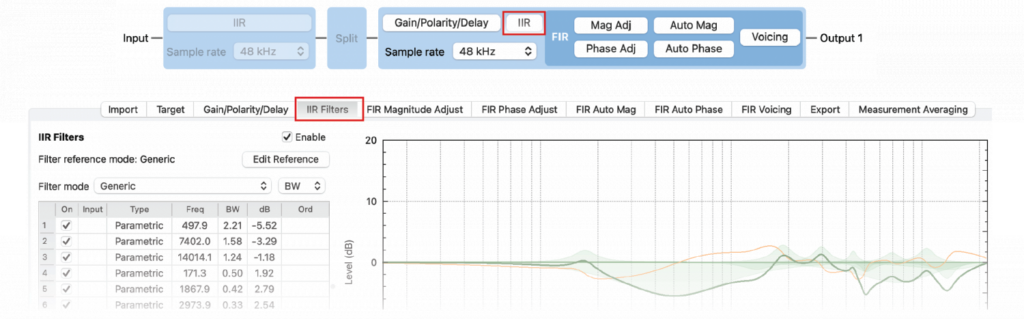
What follows is a logical, methodical process for deploying just enough filters to get the job done. I’ll use FIRDesigner (Figure 1) to generate the IIR PEQ filters for the DSP. Yes, FIRDesigner can also produce IIR filters.

EQ Workflow – Prioritized

Here’s a useful method for deploying parametric filters (PEQ). It’s based on the principle of limit what you observe, to what you can correct.

Figure 2 shows the measured loudspeaker response. The room reflections have been removed with an appropriate time window, leaving the direct field response.

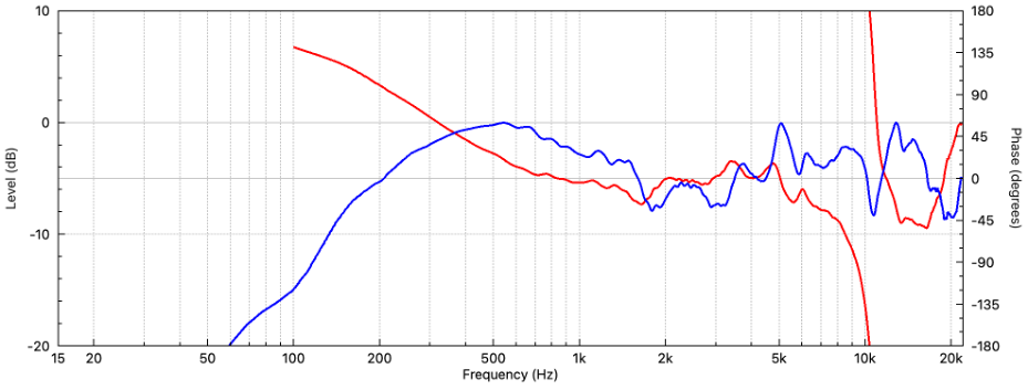
The windowing was done in the measurement program (Clio12) and the anechoic response saved an imported into FIRDesigner. Let’s neutralize it. For this article the workflow is:

Measurements – Clio 12 / Filter Generation – FIRDesigner / Filter Deployment – QSC Q-SYS

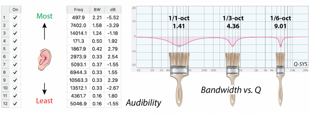
I’ll begin by smoothing the response at 1/1-octave resolution (Figure 3). This produces a much-simplified curve for deploying filters. I’ll enable a PEQ and set its bandwidth (BW) to 1/1-octave to match the smoothing.

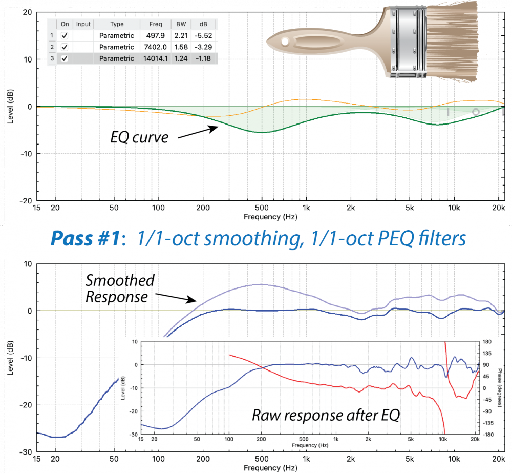
This gives us a broad filter to apply to a smooth curve. Match the filter to a bump or dip, tweak the BW as needed, and repeat until the response is reasonably smooth. Use as many filters as are needed, but as few as possible.

Next, I’ll change the smoothing to 1/3-octave (Figure 4). The loudspeaker’s response curve has more detail. I’ll enable a PEQ and set its bandwidth to 1/3-octave to match the smoothing. This gives us a more narrow filter to apply to a more detailed curve.

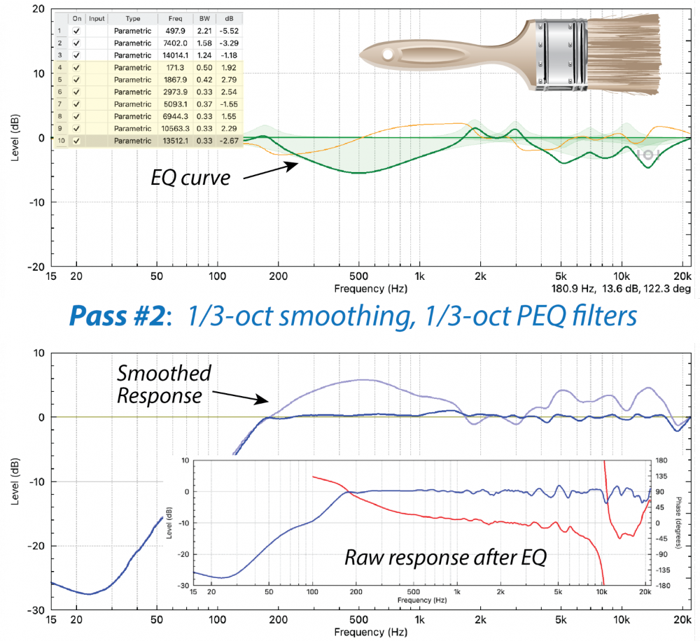
Match the filter to a bump (or dip), tweak the BW/Q as needed, and repeat until the equalized response is sufficiently smoothed. Use as many filters as are needed, but as few as possible.

The entire process can be repeated at 1/6-octave (or even higher) depending on how many filters (and how much time) are available (Figure 5).

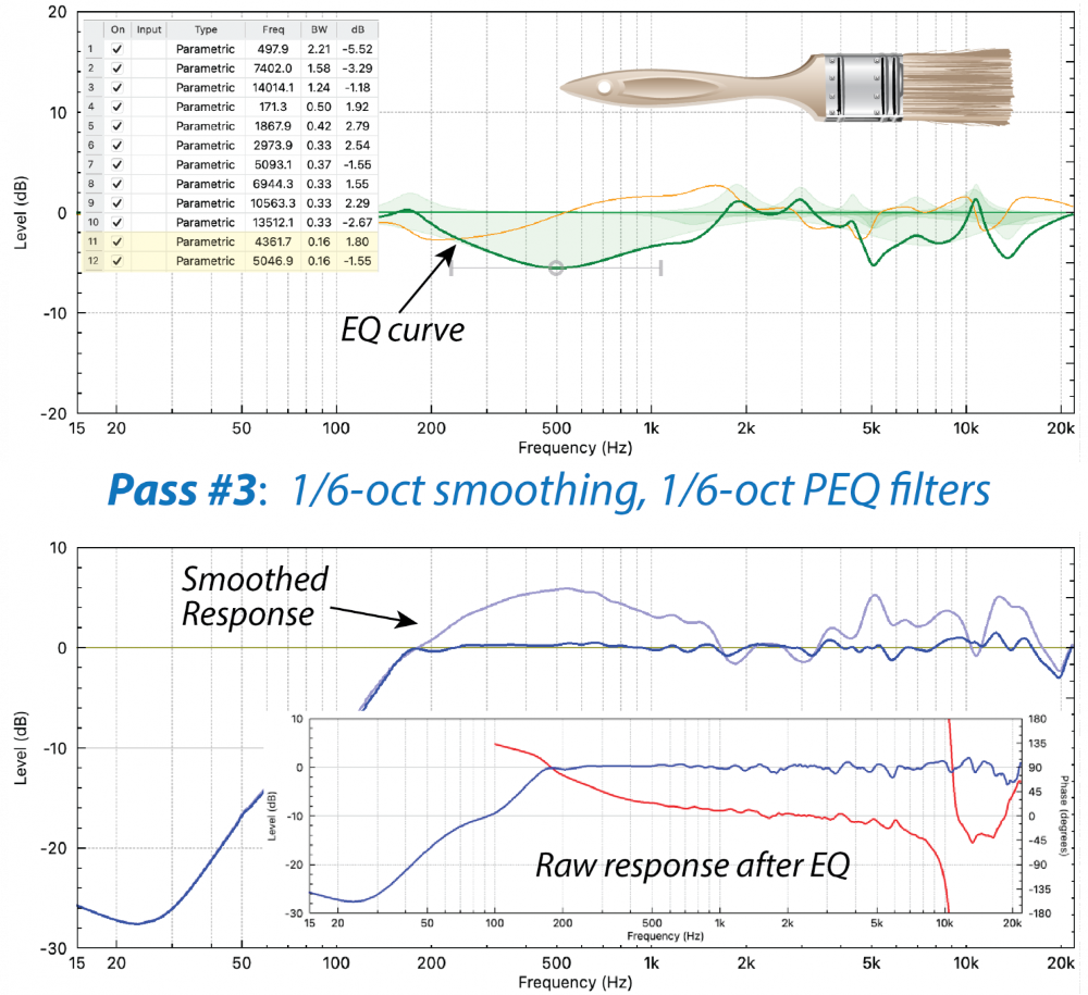
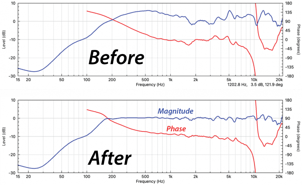
Be sure to listen as you add filters. The 1/1-octave filters will be the most audible. The 1/3-octave filters will be more subtle. Narrower filters may not be audible at all. When you reach that point you are finished! (Figure 6) Pat yourself on the back and pack up your gear.

If you use this method, the list of PEQ filters will be roughly in order of audibility – the broadest filters at the top and the narrowest filters are at the bottom (Figure 7). This is good housekeeping and useful when perusing the list and forming an idea of what the curve looks like.

Cut, Boost Or Both?

This is a common question when deploying filters. As always, the answer depends on the specific situation. I’ll offer some guidelines.

We’re after a curve “shape.” It’s irrelevant to the loudspeaker and listener whether you boost or cut to get it. Just keep in mind that with proper gain structure the signal level is closer to the top of the dynamic range (clipping) than the bottom (noise). For that reason, don’t go crazy with boost filters.

For a bi-amped or tri-amped loudspeaker, the input signal is divided between the output channels of the DSP. If you use too much cut you may not have sufficient signal level to drive the amplifier. For that reason, don’t go crazy with cut filters.

I suggest target curve with an average response at 0 dB. This will require a combination of boost and cut filters to equalize.

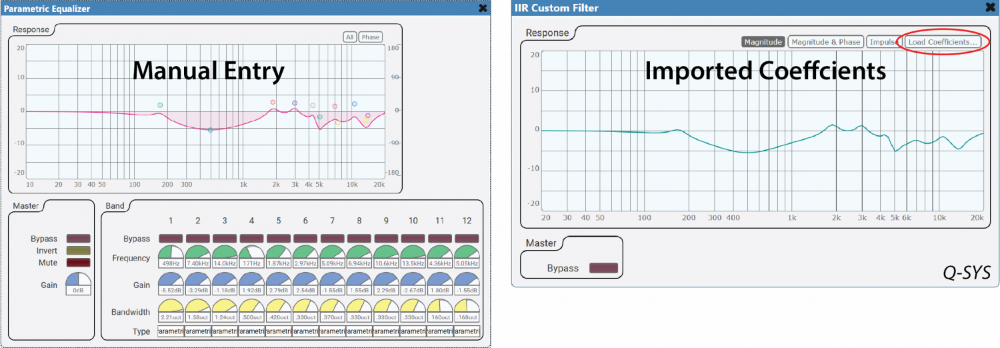
The list of PEQ filters can be transferred manually to any DSP. Some platforms allow the exported IIR coefficients to be imported into an IIR filter block (Figure 8). This is a great time-saver, but you will sacrifice the ability to tweak the individual filters within the DSP block.

Cross-Platform

In this article, I performed the entire equalization process in software. In practice you can use whatever tools are available. Nearly all measurement platforms provide smoothing functions. It makes no difference whether you are using a real-time transfer function (e.g., Smaart, SysTune) or shoot-and-look (EASERA, ARTA, Clio, REW, etc.). The process is the same.

Conclusion

Ordering the EQ workflow based on smoothing and filter bandwidth presents a logical, orderly way to equalize a response using the fewest filters possible. The system tech is free to choose between a coarse tuning and one that is more detailed. It’s like a painter who starts with a large brush and works toward a smaller one to achieve the desired level of detail.