Directivity & Angular Resolution [1]
When creating modeling files, we must know how the loudspeaker radiates sound into 3D space, meaning we must measure the off-axis radiation in order to characterize the loudspeaker’s directivity response.
To do this accurately, angular resolution must be finer than the lobes and nulls that the loudspeaker radiates.
In other words, the spatial sampling interval must be finer than the spatial attributes of the directivity. This can be likened to the sampling frequency for an audio signal. If there are frequencies higher than one-half the sampling frequency in the signal there will be aliasing in the result.
Similarly, if the spatial (angular) sampling does not have at least two measurement points for a lobe or a null, the measurement data will suffer from spatial aliasing.
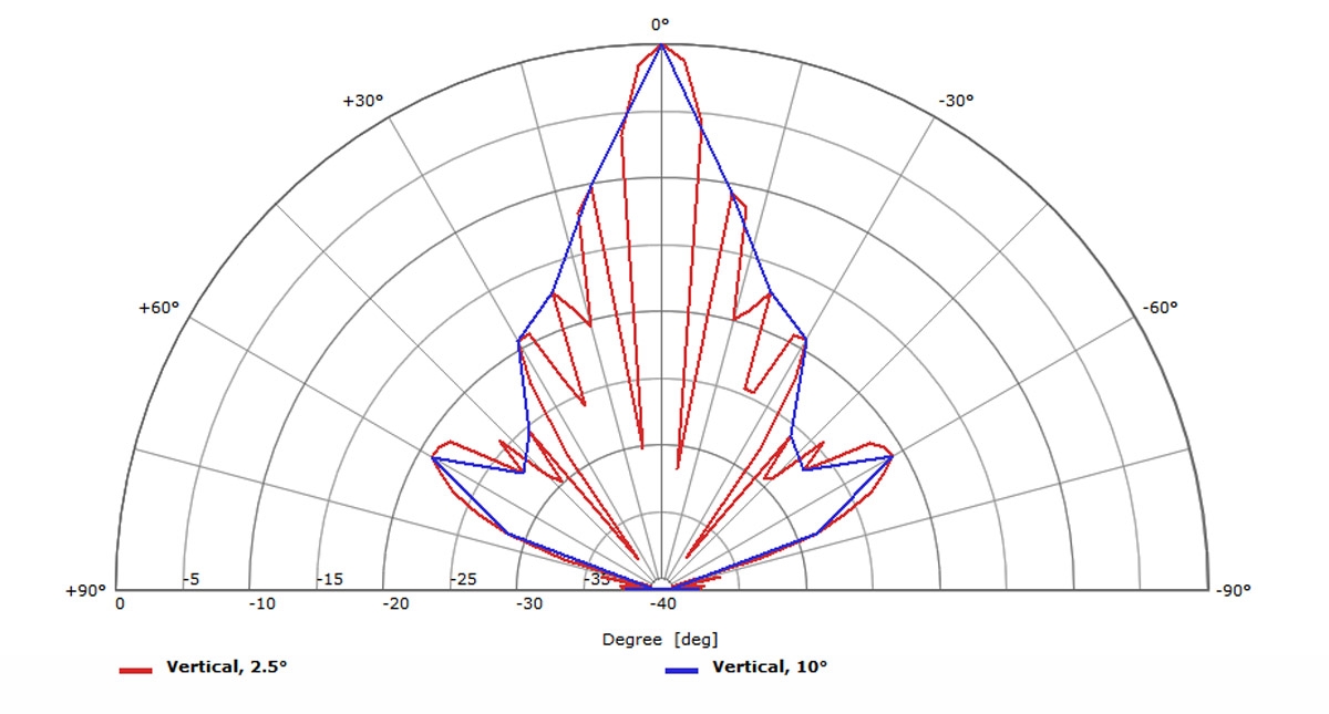
Figure 3 shows polar response plots for a line source device measured at 10-degree resolution and at 2.5-degree resolution. It’s clear that a spatial sampling of 10 degrees isn’t sufficient to accurately characterize the directivity of this device. At some of measurement points for the 10-degree resolution data, the SPL is shown to be higher than it actually is, while at other points it’s shown to be lower than it actually is.
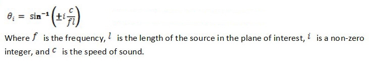
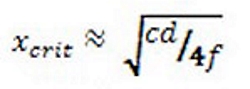
So how can we know what angular resolution is required before making measurements? The off-axis angles at which nulls occur are related to the wavelength (frequency) radiated and the dimension of the source in the plane of interest. Mathematically, this relationship is shown in Equation
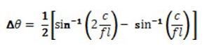
This relationship can be used to calculate the angular difference between two adjacent nulls. To avoid undersampling errors (aliasing), there must be an angular resolution for the measurements of at least half the angle between these adjacent nulls (Equation 5).
As an example, let’s say we want to accurately measure the vertical directivity up to at least 10 kHz for a ribbon driver that is 30 cm (11.8 in) tall. At 10 kHz, the first and second vertical nulls occur at approximately 6.6 and 13.3 degrees, respectively. One-half the difference between these angles is about 3.4 degrees. The angular resolution of the measurements must be at least this. If we were to measure at an angular resolution of 2.5 degrees, the data would be accurate up to about 13 kHz.
Directivity & Point of Rotation [2]
When performing off-axis measurements of a loudspeaker, a point of rotation (POR) must be selected. This is the point about which the loudspeaker is rotated so that the measurement microphone is at the desired off-axis angle. If we[re only interested in the magnitude of the off-axis frequency response, the location for the POR is not too important, within reason. However, if the measurement data is to be used for simulations in order to calculate the combined response of multiple devices, the location of the POR can be quite critical.
The reason has to do with the acoustic center (the point from which the radiation appears to originate) of the device under test (DUT). Ideally we would like for the POR to be coincident with the acoustic center of the DUT, but that’s not always possible because the acoustic center of an individual driver, much less a complete loudspeaker system, is rarely confined to a single location. That is to say, the acoustic center can change location as a function of frequency.
If our measurements contain complex data (e.g., magnitude and phase) it’s possible to deal with the POR not being coincident with the acoustic center, up to a certain point. The measured phase data can act as an error correction mechanism for the offset distance between the POR and the acoustic center of the DUT.
Note that this data must be the actual measured phase response of the DUT, not the phase response derived from the Hilbert transform of the magnitude-only data. There’s a limit to the offset distance that the phase data can effectively handle, which can generally be stated as a maximum of one-quarter wavelength at the highest frequency of interest.
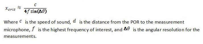
This limit for the offset distance, which has been termed the critical distance, manifests itself in the form of two different criteria. One is based on the measurement distance (the distance between the POR and the measurement microphone) and the other is based on the angular resolution used for the off-axis measurements. Each of these criteria are shown in Equation 6 and Equation 7, respectively. The lesser of the two values for the critical distance will be the governing value for the critical distance.
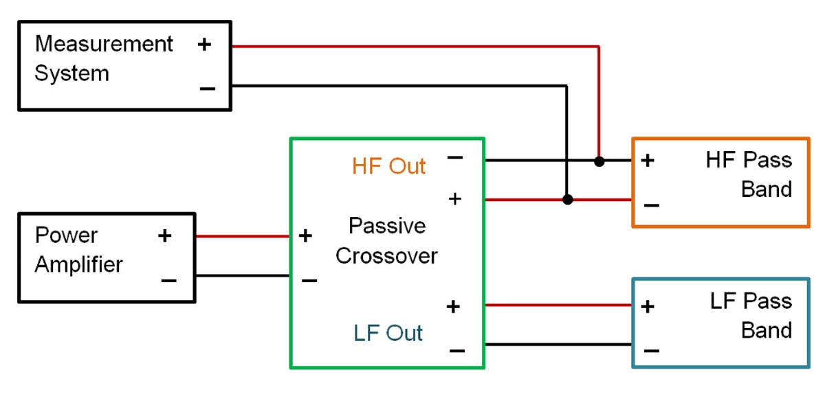
Let’s look at an example selection of the POR for a set of directivity measurements, using the same loudspeaker shown in Figure 1. This is a 2-way loudspeaker system with a 12 dB/octave passive crossover at a frequency of about 1.2 kHz. We want to be able to accurately model this loudspeaker in clusters/arrays up to about 10 kHz, and will be measuring at a distance of 4 m using an angular resolution of 5 degrees.
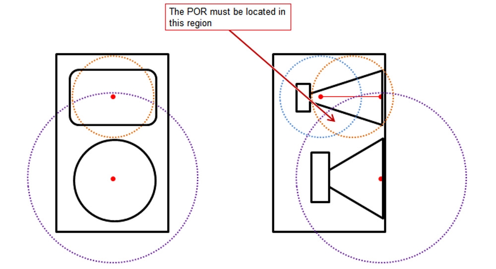
From this information we can calculate the critical distances from the woofer’s acoustic center and the horn’s acoustic center. The radii for these distances will define spheres, shown here as circles, around the acoustical center of each radiator. The area where the circles (spheres) intersect is where the POR must be located for our measurements (Figure 4).
The highest frequency of interest for the woofer is about 4.8 kHz — 2 octaves above the crossover frequency. If the crossover used higher order filters (steeper slopes) the woofer would not be radiating to as high of a frequency.
Using the other values stated above gives us a critical distance (xcrit) of 0.268 m (10.6 in) based on the measurement distance of 4 m and a critical distance of 0.206 m (8.11 in) based on the angular resolution of 5 degrees. Since the smaller value governs, the critical distance for the woofer is 0.206 m. The purple dashed circle in Figure 4 denotes this. It has a radius of 0.206 m, centered at the acoustic center of the woofer.