The highest frequency of interest for the HF horn is 10 kHz, as this is the upper limit frequency for our modeling. Using the other values stated above gives us a critical distance (xcrit) of 0.186 m (7.32 in) based on the measurement distance of 4 m and a critical distance of 0.098 m (3.68 in) based on the angular resolution of 5 degrees.
Since the smaller value governs, the critical distance for the HF horn is 0.098 m, denoted with the orange dashed circle in Figure 4. It has a radius of 0.098 m, centered at the acoustic center at the mouth of the HF horn.
Note in the side view of Figure 4 that the acoustic center can move from the mouth of the horn towards the throat of the horn at higher frequencies. The critical distance around this acoustic center closer to the throat of the horn is shown by the blue dashed circle. The entire range of locations for the HF horn’s acoustic center must be considered.
The point of rotation for the off-axis measurements must be located where all of these circles intersect. Keep in mind that the POR and acoustic centers are actually defined in 3D space so the circles represent spheres of the same radius as the circles shown.
Crossover Measurements
When the individual pass bands of a loudspeaker system are measured separately, with no filters in place, there’s also need to measure the crossover filters that will be used with the loudspeaker so they, too, can be included in the modeling file. It’s a relatively straightforward process to measure the crossover outputs but there are some things that must be considered.
These measurements must contain complex data, both magnitude and phase. If they;re magnitude-only, the resulting summation of the individual pass bands will not be correct, so a transfer function measurement must be performed.
Here again it’s important that the measured phase response is used and not the Hilbert transform of the magnitude-only data. If an active or DSP-based crossover uses delay for some pass bands, this delay must be included in the phase response. Only the measured phase response will contain this. The Hilbert transform will just have the minimum phase component and not the complete phase response.
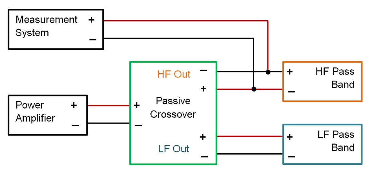
For measuring the transfer function of a passive crossover, it’s best to measure at the input terminals of the driver(s) for each pass band. This gives an accurate representation of the signal present at the input of each pass band. Since a power amplifier is typically required to drive the input to the passive crossover, care should be taken when setting the output voltage from the amplifier. An rms voltage of 1 V is probably a good starting point; the inputs of most audio analyzers should be able to accommodate this voltage without any problems.
The polarity of the measurement data must be maintained compared to the polarity of the signal at the input to the loudspeaker drivers. That is to say, the positive lead of the measurement system should be connected to the positive input terminal of the driver and the negative lead of the measurement system should be connected to the negative input terminal of the driver. If not, the polarity of the transfer function measurement will be reversed, which can cause errors in the simulations using this data.
It’s strongly recommended that only ground-isolated, balanced inputs be used for measuring crossover outputs, particularly passive crossovers. It’s not uncommon for passive crossovers to have an intentional polarity reversal for one or more of the outputs as part of the intended design.
This is shown in Figure 5, where the HF output of the crossover is reversed polarity. If a measurement system with a grounded, unbalanced input is used to measure a crossover output having reversed polarity, the positive output of the amplifier driving the crossover will be grounded. This will result in the output of the amplifier being shorted to ground. Not good!
Hopefully this discussion has provided some ideas about how to make good measurements for use in loudspeaker modeling data files. Next time I’ll take a look at using modeling files to help design a crossover for optimum directivity response through the crossover region.
References
Some of the material presented in the referenced sections was originally published in the presentations at AES Conventions and the Journal of the Audio Engineering Society. For more details on these topics please see these papers:
[1] S. Feistel and W. Ahnert. “Methods & Limitations of Line Source Simulation”, J. Audio Eng. Soc., vol. 57, No. 6, p. 379 (2009 June)
[2] S. Feistel and W. Ahnert. “Modeling of Loudspeaker Systems Using High-Resolution Data”, J. Audio Eng. Soc., vol. 55, No. 7/8, p. 571 (2007 July/August)