
Strewn across the fields of true technological and artistic credibility, the world of pro audio is littered with misinformation, overhyped irrelevance and useless complexities. Sorting through the debris to distill useful and accurate concepts can be quite challenging.
Whenever possible, I devise comparative test methods to prove or unravel various theories and assumptions. Rather than meticulously documenting the results, I opt for constructing and sharing simple repeatable test methods so that anyone who wishes to repeat the results can independently repeat them. My goal is to create a road map that allows me and others to make better audio decisions.
Over the years I’ve learned that no matter how simple or solid my tests and conclusions prove to be, there will always be counter opinions and beliefs. Or, in other words, other routes to reach similar or differing goals. I kind of like this, and it falls in line with the observation that there is often no true “right or wrong” in audio. Here are some observations and theories that have proven useful to me.
Our ears seek tonal balance. On the surface this concept is obvious and simple to demonstrate. Fire up a 15-inch, 2-way stage monitor at a relatively high volume level, and then mute the 15-inch woofer, leaving just the horn/driver on. Ouch! Without the low frequencies, the high frequencies hurt our ears – but when low frequencies are present and at a balanced volume level – the sound is no longer painful.
Expanding on this concept is the foundation behind equalizing sound systems utilizing pink noise to achieve a flat response. What may not be readily apparent is that the wider the bandwidth of the system, the louder it can be without being perceived as painful. Put into practical usage, this means that by extending the low-frequency response of a sound system, you can also turn it up a bit louder while it can still sound tonally balanced and enjoyable.
Perceived “flat response” is distance related. I believe this theory is extremely important. Not unlike perceptions of the flatness of the earth shift to a curvature, and then to a sphere as the viewing distance is increased, the sound we perceive as flat seems to change with distance as well. By “flat” I’m referring to “tonally balanced sounding.”
Many years ago, Harvey Fletcher and Wilden Munson came up with a curve showing that the tonal balance our ears perceive is volume dependant. Basically, the Fletcher-Munson curve indicates that sound is perceived as “brighter” at higher volumes. Or conversely, music that is tonally balanced at a higher volume level is perceived to lack both lower and higher frequencies when played at lower volumes.
It’s been my experience that a similar phenomenon occurs with distance. This is pretty easy to demonstrate, but I’m not sure as to the exact reasons why. In a recording studio control room, where the distance from loudspeakers to listener is relatively short, tonally balanced music that sounds smooth (and not harsh) to most people will show up relatively flat on a real time analyzer.
Conversely, with a large scale sound system measured at distances of hundreds of feet, if the music is EQ’d to flat, it will be painfully bright sounding. Knowing this is very useful for equalizing large-scale systems. Perhaps it’s that our ears expect a dulling of sound with distance, or maybe our ears act like a cardioid microphone, boosting low frequencies in closer proximities. Either way, I find that knowing to EQ “duller” for longer distances is valuable information.
We perceive tonal balance averaged over time. Returning to the earlier discussion of the painful HF that can occur when muting the LF, let’s now alternately mute the LF and then the HF.
If we do this slowly, the sound switches between bright and muddy, but if we do it more quickly, the “bright-dull” swaps begin to sound more – tonally – like a familiar kick-snare beat, which many of us rock music humans tend to find appealing.
The question is how rapidly we need to do the switching back and forth before our ears tell us it sounds O.K. Clearly this example has little realworld application, but what it highlights is that the averaging time we apply to real-time analysis systems is very relevant.
With music as a source, utilizing too slow of an averaging time can result in measured sound that looks “correct” but in reality, it alternates between sounding uncomfortably bright and overly murky. On the other hand, setting the averaging time too fast and short term can inspire us to EQ out frequencies that are not actually a tonal issue. My experience has been that an averaging time of 6 to 10 seconds provides a very useful visual readout that allows us to fine-tune the system EQ in real time while the artist is performing.
Comb filtering is not an issue with spaced sources. One of my pet peeves is that too much attention is paid to attempting to resolve comb filtering issues from separated sonic sources. Comb filtering occurs when two spaced sources are reproducing the same signal. When measuring a stereo system with a mono source signal, it’s all but impossible to get credible readings that parallel what our ears perceive.
Audio test gear will show a series of peaks and nulls, yet to our ears, it just sounds like sound coming from two places. This is not to say that comb filtering isn’t a major concern with sources in
close proximity or with lower frequencies, but on the other hand, if we test just one side of a stereo system at a time, we lose the ability to measure the combined coverage and see issues that are significant. So, what can we do to get our test gear to give us useful measurements of a stereo system?
Surprisingly there is a very simple (but rarely implemented) method. Rather than utilizing a mono random pink noise source, instead deploy two separate random pink noise sources. Even though the sources are tonally identical, because they’re independently random, they’re not the same signal. As a result, there will be not be comb filtering when running one pink source to the left side and the other to the right side.
For measuring low-frequency coverage, pan the two pink sources to the center, and for the most useful all-around measurements, I’ve found that panning the sources to about the 10 o’clock and 2 o’clock positions works well.
It’s my hope that these observations are helpful. But as with anything, check it, test it, refine it, and then bump it up a notch.
Check out Dave’s latest video, the first in a new series entitled “Sound Tips For Engineers” —