In The Field
That concludes our whirlwind tour of the basics of linearity in audio systems. And, fortunately, we know we have good tools at our disposal to isolate and measure deviations from linearity in audio systems. Sound level meters and spectrum analyzers give us good information about the real-time performance of an audio system at one measurement point, whether at a mic location or a point in the signal path, but they don’t make input-to-output comparisons.
It’s really the modern dual-channel FFT analyzer that gives us the powerful tool to make comprehensive comparisons in both frequency and time domains. By applying various test signals – noise, swept sine tones, fixed sine tones, multiple fixed sine tones, and pulses – we can isolate and measure potential non-linearities in an audio system.
Using these concepts and tools, we can set out to design and manufacture linear audio systems, and then configure, tune and operate them to perform in a linear fashion.
But first we need to define the operating parameters. Are we talking about linear performance only in the digital or analog electrical domain, or also in the domain of acoustical sound pressure? And do we need linearity across the entire audio bandwidth, above and below it as well (some say we do), or only a portion of it?
If we stay completely in the realm of signal recording and electrical amplification, audio systems have become remarkably linear in recent decades. Digital recording and mixing systems, when used within their wide but strictly defined operating parameters, exhibit a degree of linearity unheard of 50 years ago. (Outside those parameters, their non-linearity is off the charts.)
Recently, modern audio amplifiers as a rule are exceptionally linear. Progress has also been made to better convert electrical voltage to the acoustic realm of sound pressure in air, but this is an area where the limits of linear behavior are still often encountered.
But before we examine that in detail, let’s consider the elements of our complete sound reinforcement system and set some parameters within which we expect to maintain a linear relationship between signal input and acoustic output.
For our purposes here, we’ll assume that all the “artistic decisions” have been made, and we’re taking the signal from the main output of a mixing console. From here on out, the goal is to transfer that electrical signal into an acoustical signal at the desired level throughout the intended listening area, without changing anything.
To accomplish that, the signal first must pass through some kind of signal distribution, crossover and limiter devices, either in the analog or digital domains. By the time we get to the power amplifier, we must by necessity return to analog, as loudspeaker drivers (and subsequently our ears) remain stubbornly analog.
Then, assuming an active multi-amped system, the power amplifiers outputs connect to the mechanical motors of the loudspeaker drivers. These drivers, in turn, are mounted in cabinets with a specific acoustical environment defined by cabinet volume, baffling, ports and waveguides (Figure 11).
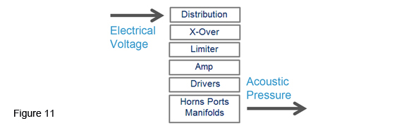
It’s at this transition stage between electrical voltage and acoustic pressure where linearity becomes particularly problematic, and the higher the SPLs involved, the more difficult it is to maintain linear behavior. For contrast, think of a condenser microphone, in which a capsule diaphragm need move only a few micrometers to generate a few millivolts of signal. Even a relatively inexpensive condenser microphone can exhibit excellent linearity.
Compare that to a high-power loudspeaker system, where an amplifier can pump peaks of around 200 volts and 80 amps into a stiffly mounted 18-inch loudspeaker, moving it rapidly several inches. Maintaining linearity here is not easily so easily accomplished, and requires a good bit of creativity along with diligent engineering.