Testing Procedures
Now that we’ve moved into the realm of audio, we need to consider measurement tools and develop some procedures to test for linearity.
At the most basic level, of course, we can simply insert a sine wave test tone and use an oscilloscope to plot the signal amplitude and display the time required to complete one cycle. Or we could use a simple spectrum analyzer, which would display amplitude over the frequency as a line or bar.
A more sophisticated approach employs dual-channel FFT transfer measurements. This is a tool which, when properly used, can reveal shortcomings in any or all three of the main linearity requirements.
Transfer function measurements, using full bandwidth signals, can be used to qualify scaling and superposition (summing) properties of a system as well as the timing aspect of homogeneity. High resolution spectral analysis of single or multi-frequency tones can be used to readily identify system shortcomings in homogeneity which manifest as distortion products.
Theoretically, we could do all our testing using single tones and laboriously plotting the results. But it’s usually much faster to use broadband noise or program content with a spectrum analyzer, which looks at the full range of frequencies in real time.
However, this does not show the time relationship. By using dual-channel analysis you can look at the complex transfer function of the system, the difference between what was sent and what was delivered (Figure 8).
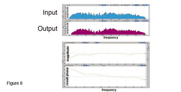
FFT analysis also lets us look at relative phase differences over a frequency range, to see if we are achieving linearity in the time domain. This is extremely useful in the time alignment of multi-way loudspeaker systems.
Finally, dual channel FFTs let us analyze the relative arrival time of energy. Do all frequencies present at the input arrive at the test microphone at the same instant, or do they spread out over time, with the system producing some frequencies later than others?
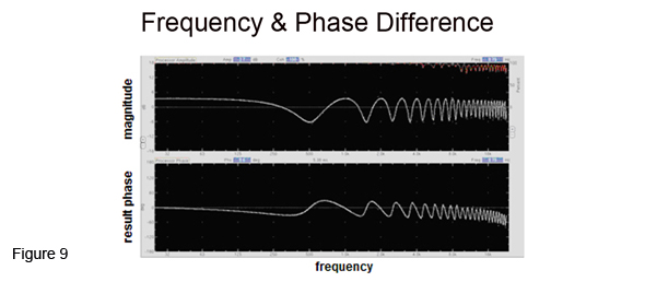
If there is a time offset between two signals, this will cause changes of magnitude across the spectrum, as signals at some frequencies will add as others will cancel. A typical example is the comb filtering caused by the relative phase differential between two signals. When two time offset signals are summed, their combined response looks like this (Figure 9).
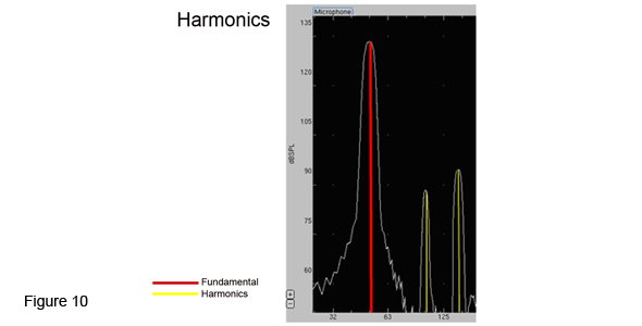
Spectral analysis reveals other differences between input and output signals, such as the harmonics generated by a loudspeaker. In the example shown here, a 50 Hz signal is being sent and the level ratio of the fundamental versus the harmonics can be quantified. The more non-linear the loudspeaker is, the closer in level the harmonics will be to the fundamental (Figure 10).