
The Clean Wireless Audio RF Mic & Wireless IEM Signal Strength Calculator is very helpful in the design and use of installed or touring wireless systems. It provides a comprehensive list of quantifiable values, imperative to the successful and legal deployment of RF systems. (The calculator is located here.)
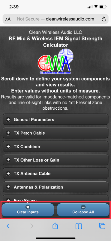
Please note the two blue bars that are ever-present at the bottom of the screen. By clicking “Clear Inputs” you will instantly erase all the information you’ve entered up to that point. “Collapse All” will close all open menus.
Here I’d like to take you through the process of using this handy tool, using a Shure Axient wireless handheld microphone system in this example.
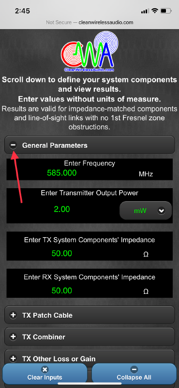
“General Parameters.” Click “+” to open the menu. Here we define the parameters of the RF system.
“Enter Frequency.” Enter the operating frequency of the mic or, for a general view, the center frequency of the systems range. To change the preset frequency, click “Enter Frequency” and a cursor will appear. For our project we will leave the frequency at the preset of 585.000 MHz.
“Enter Transmitter Output Power.” This may be a fixed or selectable option. Note the dropdown menu to select the desired measurement scale defaulted to “mW.” We will use 2 mW.
“Enter TX System Components’ Impedance” and “Enter RX System Components’ Impedance” can remain at 50 ohms. The wireless systems we use are 50-ohm systems.
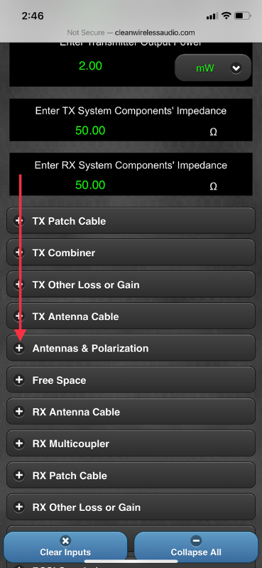
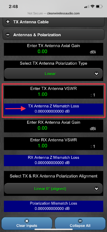
As our TX or transmitter system is simply a microphone, we can look past the TX menus. If we were using a point-to-point or IEM system, we would make entries here. Let’s move on to “Antennas & Polarization.”
“Enter TX Antenna Axial Gain” refers to the gain naturally created by the design of the antenna. The user guide will often have this information. Our microphone has a linear antenna and does not offer much in the way of extra gain. For “best case scenario” results add 1 dBi of gain. For “worst case scenario” type of result, leave it at 0 dBi, which we’ll do here.
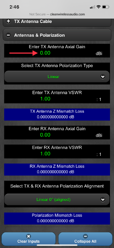
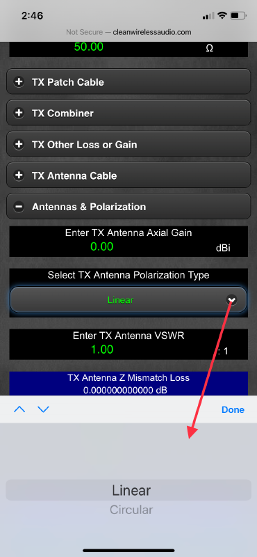
“Select TX Antenna Polarization Type.” The polarization of our mic’s antenna is “Linear.” Some of these antennae are actually circularly polarized (CP), but their design causes them to behave as linear.
“Enter TX Antenna VSWR.” VSWR stands for Voltage Standing Wave Ratio. The most signal is passed when the impedance of the components match at 50 ohms. Ohmage is measured not just in the cable, but in the connectors, splitters and most every other part of the system.
When a mismatch occurs, power is reflected back down the line causing standing waves. It’s not uncommon for components to have some reflection and their VSWR can often be found in the user guides. A VSWR of 1:1 is considered perfect, no loss. If the VSWR is unknown and you’re using brand-name professional equipment, you can leave this value at 1:1.
For our purposes, we’ll leave the VSWR of the TX mic at 1:1. Note that the calculator will provide a subtotal for the entry. This total can be found in the blue strip just below: 0 dB.
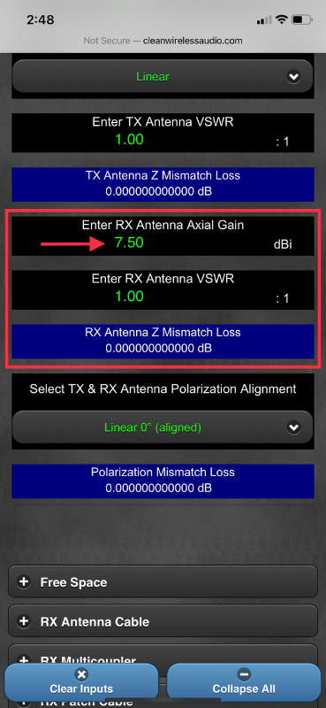
“Enter RX Antenna Axial Gain.” Let’s assume we are using the Shure UA874 paddle, which has a 7.5 dBi gain. We’ll enter that number.
“Enter RX Antenna VSWR.” The manufacturer does not specify a VSWR for this so I’ll leave it at 1:1.
“Select TX & RX Antenna Polarization Alignment.” This is asking how the RF signal propagates from the antenna and how the antennas are aligned to one another. A “whip” or “rubber duck” and paddle antenna propagate in a linear fashion, while a CP or “helical” antenna propagates in a circular fashion.
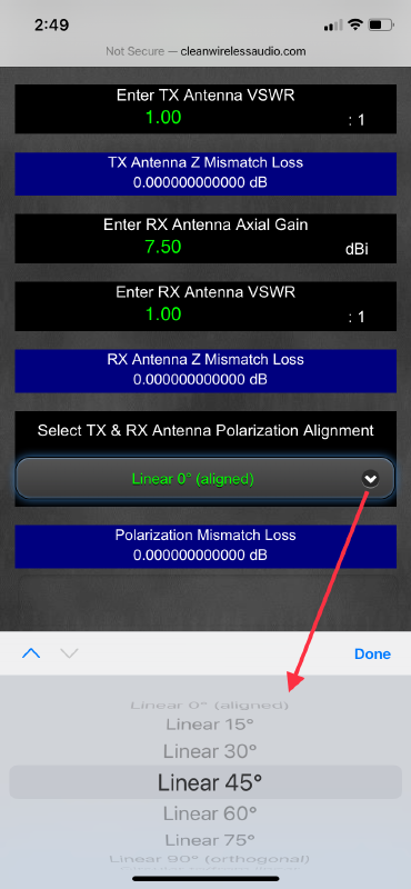
The menu selections include “Linear 0° (aligned)” through to “Linear 90° (orthogonal).” If you’re using a linearly propagating antenna for both Tx and Rx, these are the selections. If the mic is perpendicular to the ground and the Shure UA874 Rx antenna is also perpendicular, they’re considered aligned and therefore “Linear 0° (aligned)” is the selection. If the mic is parallel to the ground and the Rx antenna is perpendicular, “Linear 90° (orthogonal) is the selection. Employ your best judgment if it’s between those options.
If we’re using a helical RX antenna, use the “Circular to/from linear” selection. In a point-to-point system utilizing helical antennae, we must consider the orientation of the winding. One could check the user guide for this or visually follow the path of the signal as it would travel down the copper windings of the antenna. A clockwise rotation is right hand (RH) and counter-clockwise is left hand (LH). Combining LH and RH wound helicals will cause a great loss of power.
Anyway, for this project we’ll select “Linear 0° (aligned).”
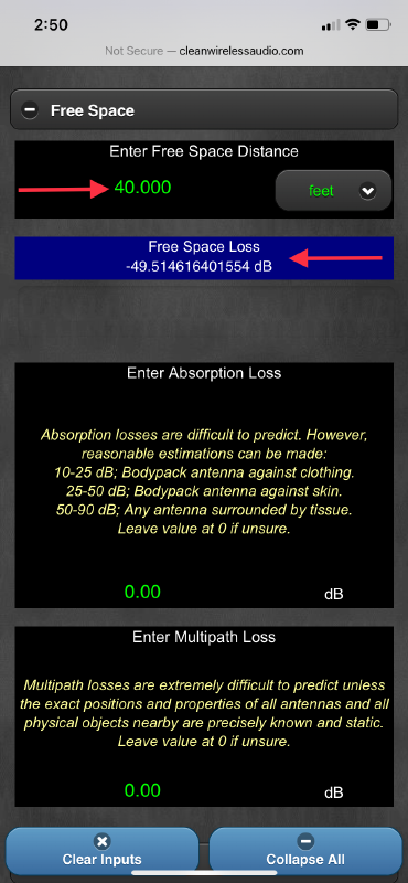
“Free Space” is the distance between the mic and the antenna. Here we’ll witness a great loss in RF power. This is the most efficient place to increase RF power and quality of reception. By moving the antenna closer to the microphone we can make great gains. “What of the loss through the cable?” you might ask. It’s a small trade-off because it’s much easier for RF to travel through copper than air.
This project will place the mic 40 feet from the antenna. Please note blue strip that shows the “Free Space Loss” subtotal at -49.5 dB. Changing the distance to 20 feet would show -43.5 dB — that’s a 6 dB difference!
If the artist were wearing a bodypack, we might need to consider absorption loss. The calculator makes note of some standard scenarios. Use your best judgment to predict the loss.
In this example, however, the artist is using a handheld mic and has good mic technique so we have a 0 dB loss.
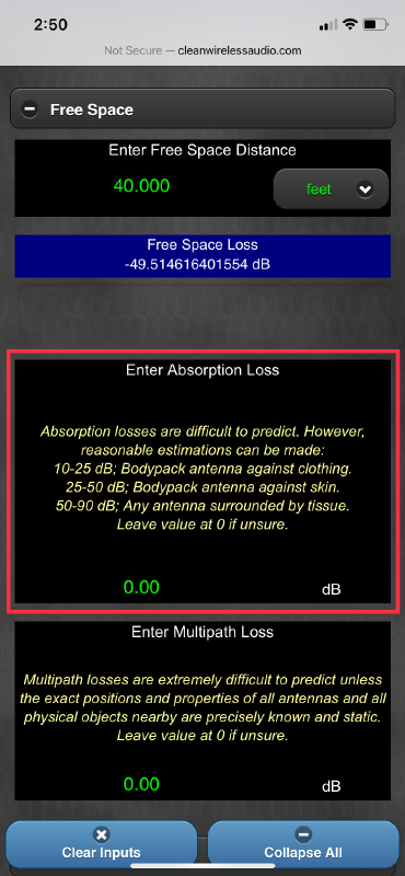
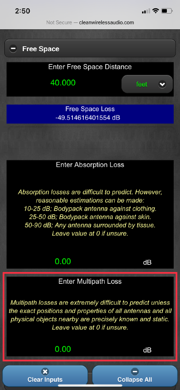
“Enter Multipath Loss” is out of the scope of this project. This section is for very advanced users. Simply put, it serves to calculate additional losses caused by static objects between the mic and antenna that reflect the signal in such a manner that it cancels a portion of the source signal. Let’s leave it at 0 dB.
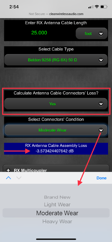
“RX Antenna Cable.” Here we define the characteristics of the cable. Start with “Enter RX Antenna Cable Length,” which is in either feet or meters, selected via the drop down menu. Let’s enter 25 feet for this project.
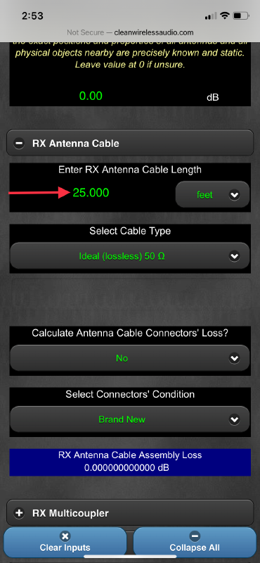
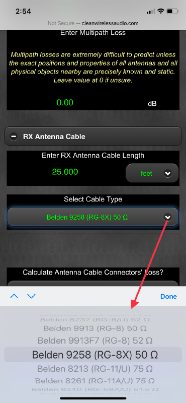
“Select Cable Type.” This can often be found printed on the side of the cable. By opening the drop-down menu we see there are a number of choices. The list begins with general cable types and then moves on to specific manufacturer cables. Our cable reads BELDEN RG8X. Looking down the list we find “Belden 9258 (RG-8X) 50 ohm,” so let’s select it.
“Calculate Antenna Cable Connectors’ Loss?” Open the dropdown menu and select either yes or no. We’ll include this calculation and therefore will select “Yes.” From here, define the condition of the connector. Clicking under “Select Connectors’ Condition” allows us to select the amount of wear of our connector.
We’ll choose “Moderate Wear” for this project. There will be a loss of 1.5 dB due to this selection, and including our loss for the cable, will bring our total “RX Antenna Cable Assembly Loss” to approximately 3.5 dB of loss. This can be seen in the blue strip.
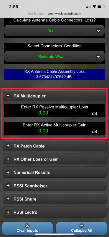
“RX Multicoupler” refers to the system’s antenna distribution system or “antenna splitter.” In this project we’ll use the Shure UA844. It’s an active splitter, and therefore, we hope to make an entry in the “Enter RX Active Multicoupler Gain.” A look at the user guide reveals this unit has a gain of -1 to +1 dB. Let’s leave the gain amount at 0 dB.
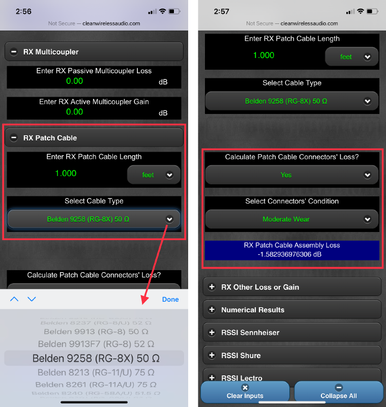
Now we’re at “RX Patch Cable.” This is the (usually) short cable linking the antenna splitter to the receiver. Here, the “Enter RX Patch Cable Length” entry will be 1 foot. We’re still using BELDEN RG8X cable. Use the “Select Cable Type” dropdown menu to make this selection.
Again, we’ll include the connectors in our calculation, so select “Yes” in the “Calculate Patch Cable Connectors’ Loss?” menu. We can specify “Moderate Wear” once again in the “Select Connectors’ Condition” menu.
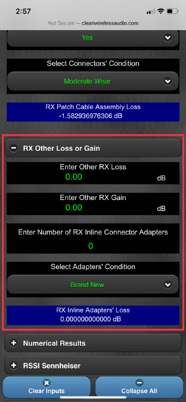
“RX Other Loss or Gain” provides the opportunity to include additional gains or losses not covered by the calculator. Perhaps we’ve extended the antenna cable and want to include the loss of the connector — this area allows for that inclusion. However, this example project doesn’t have any other gains or losses, so we can move on.
The “Numerical Results” section provides us with the total system losses (or gains) and therefore a prediction of how the system will perform. The calculations are displayed in the blue strips.

We’re measuring a microphone so we can ignore the “TX System Loss (-) or Gain” strip. The total for this strip should be 0 dB.
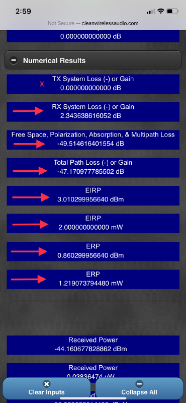
“RX System Loss (-) or Gain” shows a total of losses or gains as caused by the equipment. A loss would be indicated by a “-” preceding the number. Our system has gained more 2 dB.
“Free Space, Polarization, Absorption, & Multipath Loss” provides a total representing how the signal is affected by the environment in which it travels. We’ve lost approximately 49 dB (-49 dB).
“Total Path Loss (-) or Gain” is simply the difference between the previous two totals. We have a total path loss of approximately 47 dB (-47 dB).
EIRP (Effective Isotropic Radiated Power) and ERP (Effective Radiated Power) are very important numbers. The FCC and similar governing bodies that manage the RF spectrum have transmission power limits. This calculator provides these figures in dBm and mW.
“EIRP” shows a measurement of approximately 3 dBm or, as shown in the next blue strip, 2 mW.
“ERP” shows a measurement of approximately 0.8 dBm or 1.2 mW.
“Received Power” and “Received Voltage.” Manufacturers typically provide a sensitivity requirement in the user guide, often using one of these scales. By comparing the received power to the required amount and cross-referencing that with the RF noise floor, we can get an idea of how well the system will perform.
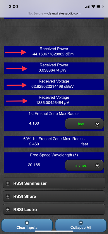
Imagine the primary wave of the RF signal in our project being a straight line from the transmitter’s antenna to the receiver’s antenna. The Fresnel zones are radiating “football-shaped” or “rugby ball-shaped” bodies of RF power around this imaginary line. The sizes of these zones are frequency and distance dependent, and they’re ever-changing as our artist moves about.
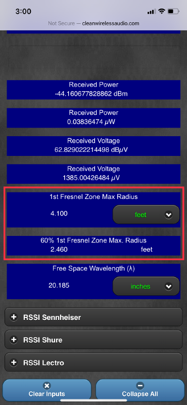
“1st Fresnel Zone Max Radius” shows a sum of approximately 4 feet. It’s best to keep this area clear of dense, reflective obstacles because any more than a 40 percent blockage can severely degrade the signal.
“60% 1st Fresnel Zone Max. Radius” provides us with an idea of how far into the Fresnel zone we can get before we begin to experience severe degradation.
If the stage is clean and open, you can probably overlook the Fresnel zone calculations. However, if there are obstacles, this may be quite important. I’ve witnessed a support group forced to place their gear far upstage, creating many reflective obstacles to be in the transmission path. If they’d used this calculator, they would’ve had a good idea of how to place their antenna.
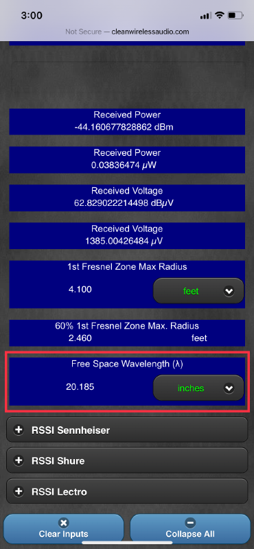
“Free Space Wavelength.” This calculation is used in antenna design, among other things, and isn’t required for our project.
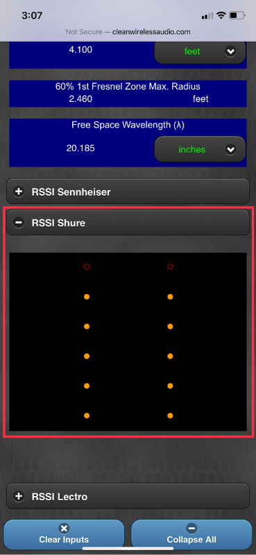
Lastly, the calculator provides our RSSI or received signal strength indication. If we click on “RSSI Sennheiser,” “RSSI Shure” or “RSSI Lectro” (Lectrosonics), we can view our predicted metering. If we click on RSSI Shure we can see that there should be very good reception. However, if the real-world results don’t match, it’s time to check for issues along the path.