ar•ray•a•bil•i•ty [uh-ray-a-bil-i-tee]: 1. The properties of a transducer, or a transducer system, that permits summation with others of like kind, thereby providing an overall increase in energy.

While this definition includes devices such as microwave and sonar antenna arrays, here I’m specifically referring to an increase in acoustical energy.

And with that, it’s fitting to say that it’s hard to find “arrayability” in most dictionaries. Even “arrayable” isn’t in most dictionaries, but both terms show up incessantly when talking about loudspeakers.

Essence Of The Issue
Sound travels quite slowly in air. This makes the arrival time, which dictate the relative phase relationship among two or more sonic sources, a critical issue in respect to how they will interact when more than one wavefront meets another.

So what makes a loudspeaker arrayable? “Any loudspeaker that is intended to be used in multiples must be carefully designed and thoroughly tested with like units to establish its viability as a member of an array that collectively provides reasonably flat constructive summation.” Well, that’s a mouthful. And unfortunately, careful design and thorough testing is not always the case.

There is a significant cost involved in building multiple prototypes, then possibly re-engineering the initial design, and then re-building and re-testing additional iterations until optimal acoustic summation has been achieved. It’s far easier (and cheaper) to predict what the array will do, rather than construct it in the physical domain and actually measure the response of various groupings of loudspeakers. And predicted response is precisely what most manufacturers concentrate on.

Let’s keep in mind that the goal of any loudspeaker array is to behave as a larger version of its individual elements. This doesn’t mean that the array cannot possess new properties of its own (and indeed it will) but rather, that the fundamental response of each array element should be constructively incorporated into the overall array response.

Sound Meets Light
It’s easy to think of sonic energy in the same way that we think of light sources: aim two or more luminaires at an object and they will collectively brighten the object more than a single lamp. Lights don’t care if they are of equal intensity, differing intensity, or widely varying distances from the subject that they are illuminating. That’s because of how incredibly fast light waves travel.

Not so with sound. In the audio domain, two or more loudspeakers focused on a given point in space may or may not produce a greater level of intensity. And even if multiple loudspeakers do increase the overall intensity, they are likely to cause all sorts of unevenness in the spectral response, thus degrading the sonic quality from that of a single loudspeaker. And that leads us to arrayability…

First, let’s establish that loudspeakers are not so easily defined as arrayable or not arrayable. In a manner of speaking, all loudspeakers possess both characteristics to some degree. In practice the issue is complex, and involves an understanding of wavelengths, pressure, and acoustic power.

Schools Of Thought
Belief System #1: Many sound system designers and audio practitioners have adopted the notion that if two trapezoidal loudspeaker enclosures with a stated angle of dispersion – let’s say 30 degrees for this example – are placed adjacent to one another at a 30-degree included splay angle (this means that the side walls of the trapezoidal enclosures are probably 15 degrees each), then the result will be a seamless 60 degree system. Or, if three enclosures are used adjacent to each other, they will form a seamless 90 degree system, and so on.

If this was as complicated as it gets, then all 30-degree loudspeakers would be the same as all others. Moreover, the total power output of the array could never be greater than that of each array module. But that’s absolutely not the case.

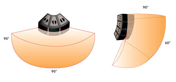
There is no such thing, in practical usage, as a 30-degree loudspeaker, nor a 45, a 60, or a 120 (though there are plenty of 360-degree loudspeakers; most are known as subwoofers). To understand why this is true, let’s look at how directivity is stated in loudspeaker product literature.

The angle of dispersion that defines acoustical coverage is almost always based on -6 dB “down” points in which the off-axis energy is -6 dB (less) than the on-axis energy. And that’s usually measured at 1 kHz, or at some frequency in which the HF horn (and MF horn, if applicable) exhibit some measure of control. But this nearly ancient way of characterizing a loudspeaker’s dispersion ignores the vast differences between LF, MF, and HF. Acoustical behavior is not cut and dried.

At lower frequencies, the LF content will get wider and wider in dispersion until it becomes essentially omnidirectional, under all but the most abnormal of conditions (think 60-foot long horns…abnormal, right?). Very long wavelengths (low “E” on a bass guitar is about 30 feet in length) need either very large horns or very large arrays to provide pattern control. Think of it like this: doing much of anything that might control LF dispersion takes a lot of building materials.

So here we have our first conundrum: the directivity pattern of a loudspeaker, thought by many to dictate what an array will (or will not) accomplish, typically varies by about two orders of magnitude from a loudspeaker’s LF range (assuming it can reproduce 40 Hz) to its HF range (assuming it can reproduce at least 4 kHz).

And that brings us to our second conundrum: an important property of dispersion, and especially how it affects arrayability of like devices, is often overlooked. The property is what happens after the -6 dB down point. A given horn might cut off drastically in amplitude, whereas another might fall off slowly and gently as the dispersion angle increases.

In other words, a horn stated to be 90 degrees at 1 kHz might provide very usable response at 120 degrees, perhaps being only -9 dB than its on-axis reference amplitude. And that could be a good thing if the response remains reasonably flat. The off-axis seating is likely to be physically located much closer to the loudspeaker than the on-axis seating, which means that additional “fringe-fill” loudspeakers may not be needed.

By contrast, another 90-degree horn or horn array might be as much as -24 dB lower at 120 degrees, making its broad-band off-axis response rather unusable. But more to the point, these widely varying horn characteristics will not behave the same when configured into an array. And this leads us to…

Belief System #2: In this second look at arrayable loudspeakers we see a smaller following among loudspeaker designers because the rules aren’t as easy to comprehend. If you put two 90 degree loudspeakers next to each other, and splay them apart at a 20 degree included angle, should you not get 90 + 90 + 20 = 200 degrees of dispersion? It would seem so. But that’s not at all what happens.

Instead, the pressure from the two or more radiating devices, that’s the horns and cones, will combine in some particular manner. Exactly how they combine is the grand issue behind whether or not they will form a useful array or conversely, are just a bunch of speakers placed near each other that combine like oil and water.

For the record, this is the belief system that Apogee Sound based its designs upon. And it really can be called a “practice” rather an a “belief system” because the patterns and response curves of the resultant arrays were exhaustively measured outdoors, 30 feet above ground level, and carefully documented using Hewlett Packard and TEF measurement equipment. It was a process that took several months of full time work.

The net value, simplified as much as possible from the exhaustive process, was that low pressure audio sources combine much more readily than high pressure sources. Stated another way, sonic energy emanating from the mouths of horns is far more amenable to summing with like units than at the throat of horns.

The New Math
So it turns out that a certain 90-degree horn sitting adjacent to another 90-degree horn – both with very gradual fall-off characteristics – actually combine together quite well. The behavior is something like an old fashioned multi-cellular horn, producing a summed output that is on the order of 70 degrees.

Add a third horn to the array and the -6 dB points become even narrower, about 60 degrees. Build it larger, let’s say seven 90-degree horns, and the – 6 dB points become narrower still, about 40 degrees.

But here it’s important to note that we’re focusing on -6 dB points which, as noted earlier, are the industry standard for defining dispersion angle. The forward radiated power is much greater than that of a single horn, and that’s exactly what proper arrays should accomplish.

The useful angle of coverage of this array is much wider than its forward radiated power (again, based on -6 dB points). What do we mean by useful angle? That would be any point in the overall dispersion pattern that remains reasonably flat. If only 50 Hz to 100 Hz exhibits 180 degrees of coverage, but higher frequencies are far narrower, than 180 degrees would not be considered a useful angle of coverage.

Cone-ology
Loudspeaker cones are altogether different from horns. Horns are designed to cover a certain dispersion angle. Cones are designed for everything but. The diameter and the geometry of a given cone’s flare-rate dictate the angle of coverage of an individual cone driver which, as one might suspect, will always be conical in nature.

The angles and configurations in which multiple cones are arrayed in respect to one another effect how a grouping of cone drivers will array together (and by the way, “array” is both a noun and a verb). That said, and as previously noted, in practical terms all acoustical behavior is a function of frequency.

So here we have some diameter of cone driver that will exhibit a wide pattern at lower frequencies and a narrower pattern at higher frequencies. And we wish to combine it with others of like kind. And that leads us to line arrays…

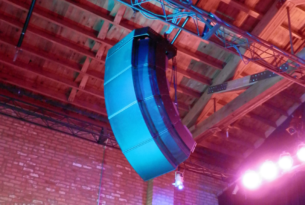
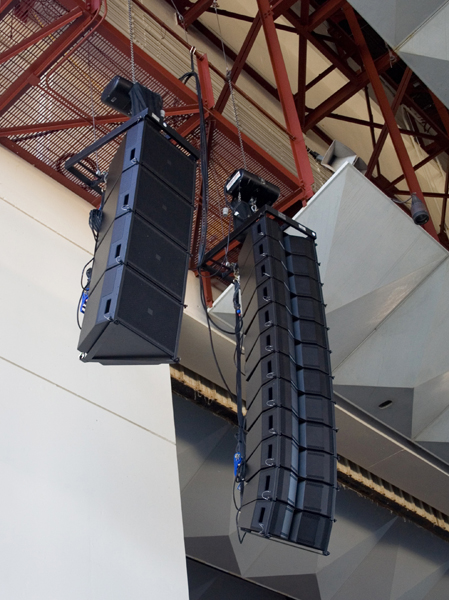
Line Array Directionality
Somewhat opposite to the concept of arraying groups of predominantly horn-loaded loudspeakers in the quest to ultimately generate large-system pattern control, the modern line array is a mixture of horns (or waveguides as many manufacturers name their devices) combined with various sizes of cone drivers.

The pursuit is clear: improved directivity and the benefit is delivering sound to the seated audience areas while minimizing ‘acoustic overflow’ into unseated regions of a venue. By eliminating unwanted reflections from walls and ceilings, the direct sound should be clearer and cleaner.

However, line arrays tend to excel at sending coherent sound over long distances which makes the reflections more of a discreet echo instead of the scattered reverb effect of less coherent systems. The trick, it seems, is to focus the line array very, very carefully to avoid discreet reflections.

There’s an easy way to explain what happens in a line array formation. The multiple sources in the line generate acoustical addition with one another, mostly because they are closely arrayed in the physical plane, while they simultaneously generate cancellation lobes off-axis. This factor forms a line array’s exceptional ability to provide tightly defined directionality in the long axis of the line.

As you walk towards a well designed line array and then walk directly under it, it will sound like the level was attenuated by a very large number. And that’s a good thing when dealing with feedback and other stage-related contamination.

Let’s look at it like this: stack up a bunch of acoustic sources in a line – curved or not – and there will be a measure of acoustic addition and a measure of cancellation. Account for the band-limited parameters that always exist in relation to the transducer sizes and shapes (with DSP no doubt), and one can create a system that ultimately provides broad-band directional control.

But it’s not so easy. Combining conical sources, such as 6- or 8-inch cone drivers in the MF range, so that they acoustically mate with HF waveguides that are designed to keep high frequency output as narrow as possible, does not make for an easy outcome.

All sorts of things are then done to try to get vastly different dispersion patterns to roughly agree with each other. Angling the cone drivers is usually the first step. The next is to provide various forms of physical baffles that interrupt the cone driver’s native dispersion characteristics. Finally, DSP is used in an attempt to manage pattern control.

The good news is that almost anything that produces sound, when combined in a closely coupled line, will take on a measure of vertical control all on its own. Thus, most line arrays, whether carefully engineered and tested – or not – will exhibit a measure of useful pattern control.

As the world of professional audio continues to grow and develop, it’s likely that a steady rate of product improvement will be on the menu. The job of the end user is to separate idle claims from demonstrable benefits. And that’s something we, as a group, do pretty well.