
Figure 4 is an FIR filter created using 48kHz sample rate and 1024 taps.
Although an FIR filter can be created as minimum phase, but what is powerful with FIR is the ability to independently control the frequency and phase responses.
This is what is commonly called a linear phase FIR filter.
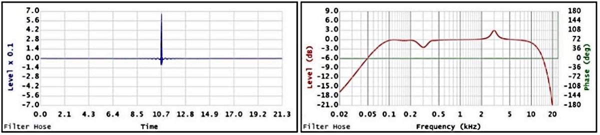
Figure 4
Figure 4 – the left graph shows the filter’s impulse response. Since the peak of the impulse response is located at 10.65ms, this shows a processing delay caused by the filter. In other words, the output will be delayed by an additional 10.65ms, which can be too long for live stage monitoring or overdub recording but can be acceptable for audio mastering or music listening use (without video).
Figure 4 – the right graph shows the transfer function of the FIR filter with the processing delay removed by cyclic shifting the impulse response for easier viewing. The reader can observe the phase response that is flat at 0deg (there is no phase shift caused by the filter) and the frequency response is similar to figure 3 – right.
Digital FIR Filter Properties
In the digital world, sample rate (fs) is one of the most limiting conditions to recognize. The FIR filter depends on the sample rate of the hardware/software. One can’t just change the sample rate of a filter and expect the same result.
As the name implies, an FIR filter has a finite duration or a certain number of taps. An FIR’s tap is simply a coefficient value and the impulse response of an FIR filter is the filter’s coefficients. The number of taps (N) is the amount of the memory needed to implement the filter. More taps mean higher frequency resolution, which in turn means narrower filters and/or steeper roll-offs.
Frequency resolution = fs / N.
By dividing the sample rate by N, a practitioner is able to calculate the frequency resolution of the filter. In the example above (figure 4), the FIR is created using 48kHz sample rate and N=1024.
This yields a frequency resolution of 46.875Hz. For a quick and rough estimation, we can multiply the frequency resolution by 3 (three) to predict the effective low frequency limit of the filter. 46.875Hz x 3 ≈ 141Hz. This means an FIR filter with fs = 48kHz and N = 1024 will be effective at 141Hz and above. This is just a quick and rough estimation based on a sample rate and number of taps, however other calculation parameters or filter editing will heavily affect the final result.
To create a steep high pass at low frequency (below 200Hz), one may require a high N value which may not be practical. Therefore it is common to implement a HPF as an IIR filter in addition to an FIR filter.
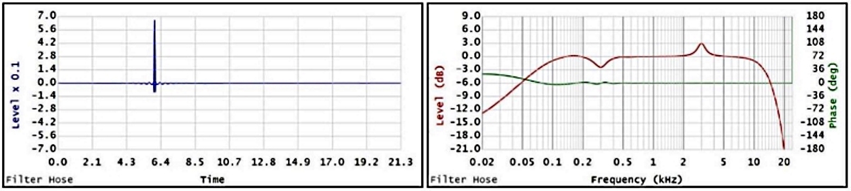
Figure 5
Filter’s Processing Delay
Another important factor is editing the filter.
Figure 4 shows the FIR filter with 10.65ms processing delay. When the location of the filter’s impulse is cyclic shifted and appropriate windowing is performed based on the new impulse location, the result filter’s transfer function may change.
Please observe figure 5 (with 6ms processing delay), figure 6 (with 3ms processing delay) and compare them to figure 4 (with 10ms processing delay).

Figure 6
All phase response curves in figure 4, 5 and 6 are observed by cyclic shifting the filter’s impulse response peak to 0ms.