I’ve designed a lot of crossovers for loudspeakers during the last 30 years, and I’m sure that many of you have also designed them. Even just dialing in the filter parameters on a DSP means you’ve designed a crossover.

An important question to ask: What are the filters doing to the response of the loudspeaker? Some of you may have measured the frequency response of the loudspeaker to determine what’s happening through the crossover region.

However, most only look at the on-axis response of the loudspeaker. It’s equally important, or perhaps more important, to know what’s happening off-axis. Let’s see how loudspeaker modeling can be used to help with this.

There are quite a few loudspeaker modeling programs that let users look at the on-axis frequency response of a low-frequency pass band (woofer) or a high-frequency pass band (tweeter or compression driver/horn). Of course, the user has to enter the measurement data for each of the pass bands.

These programs also allow the specification of different filters that are used to alter the signals presented to each of the pass bands (Figure 1).

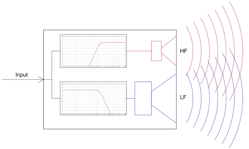
The effects of the filters on each of the pass bands are calculated, and the response of all the pass bands can then be added together to simulate the on-axis response of the loudspeaker. But what’s happening off-axis?

Let’s replace the on-axis frequency response data of each pass band with directivity data (on-axis and off-axis frequency responses) for each pass band. We can combine this data with the effect of the filters and calculate the directivity response of the complete loudspeaker system.

This may not seem like a big deal, but it can save an incredible amount of time when evaluating a crossover design. Instead of making changes to the crossover and then re-measuring the loudspeaker (which can take 30 minutes or more) in order to see the effects on the directivity of the loudspeaker, the directivity response of the system can be calculated in seconds.

Keep in mind the directivity data and the filter data must be complex data (both magnitude and phase). It also needs to be sufficiently accurate for the intended purpose (see “Executing Measurements for Loudspeaker Modeling Files”).

Looking Deeper

To illustrate this, we’ll use a two-way loudspeaker with a 15-inch woofer for the LF pass band and a compression driver on a constant directivity horn for the HF pass band. The horn is located above the woofer, vertically. This can often make for a less than ideal vertical directivity response.

The on-axis frequency response of the LF and HF pass bands, along with the combined summation, using the original crossover filters from the manufacturer of this loudspeaker are shown in Figure 2. This seems to show good summation through the crossover region (from about 1 kHz to 2 kHz).

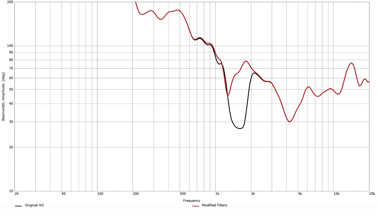
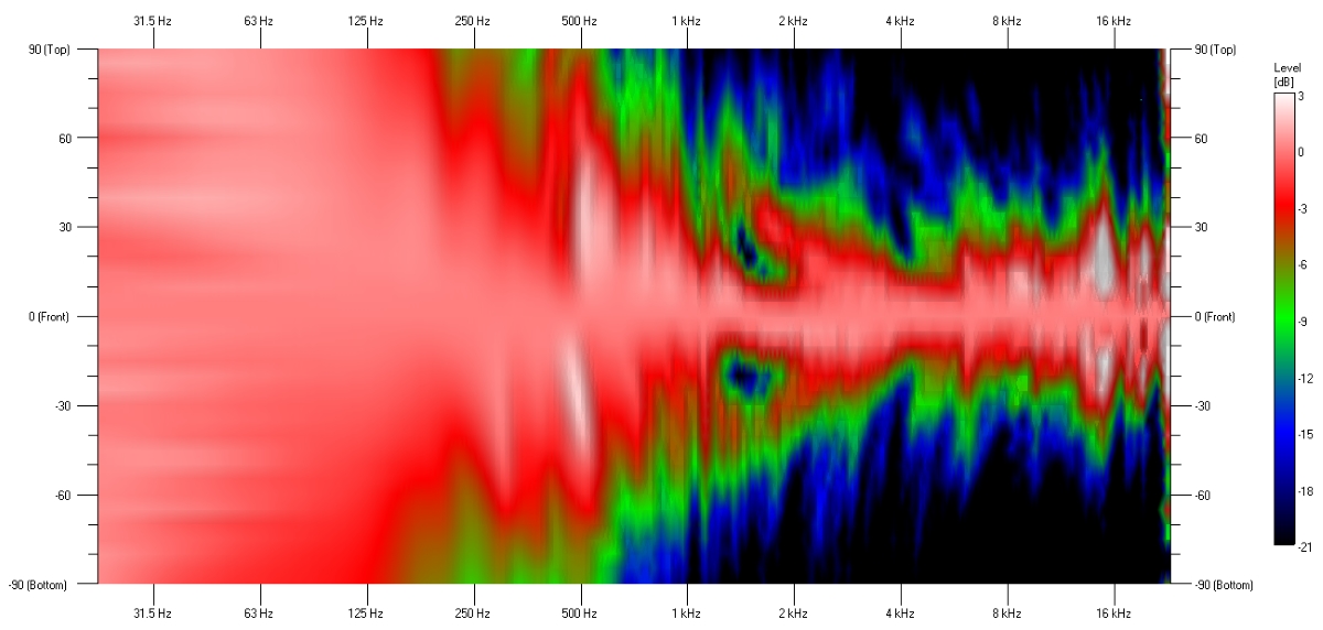
However, when we look at the vertical beamwidth (black curve in Figure 3) or the vertical directivity map (Figure 4), we see that there is a problem in the crossover region. The beamwidth, or coverage, of the loudspeaker narrows considerably from a desired value of about 60 degrees to less than 30 degrees in the 1 kHz to 2 kHz crossover region.

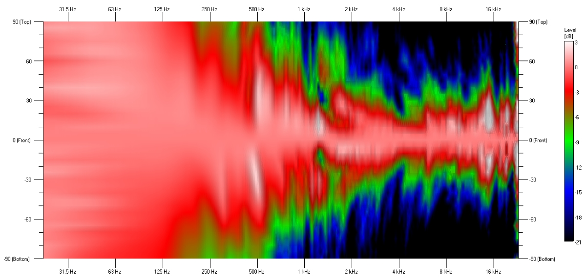
By applying a few different parametric equalization filters to the LF and HF pass bands, the vertical directivity can be improved, as shown by the red curve in Figure 3 and the vertical directivity map of Figure 5. This improvement may have taken days to realize if new measurements of the vertical polar response had been required after each tweak of the new equalization filters. By using the modeling data files for the individual LF and HF pass bands, the changes and optimization of the loudspeaker’s directivity was accomplished in a few hours.

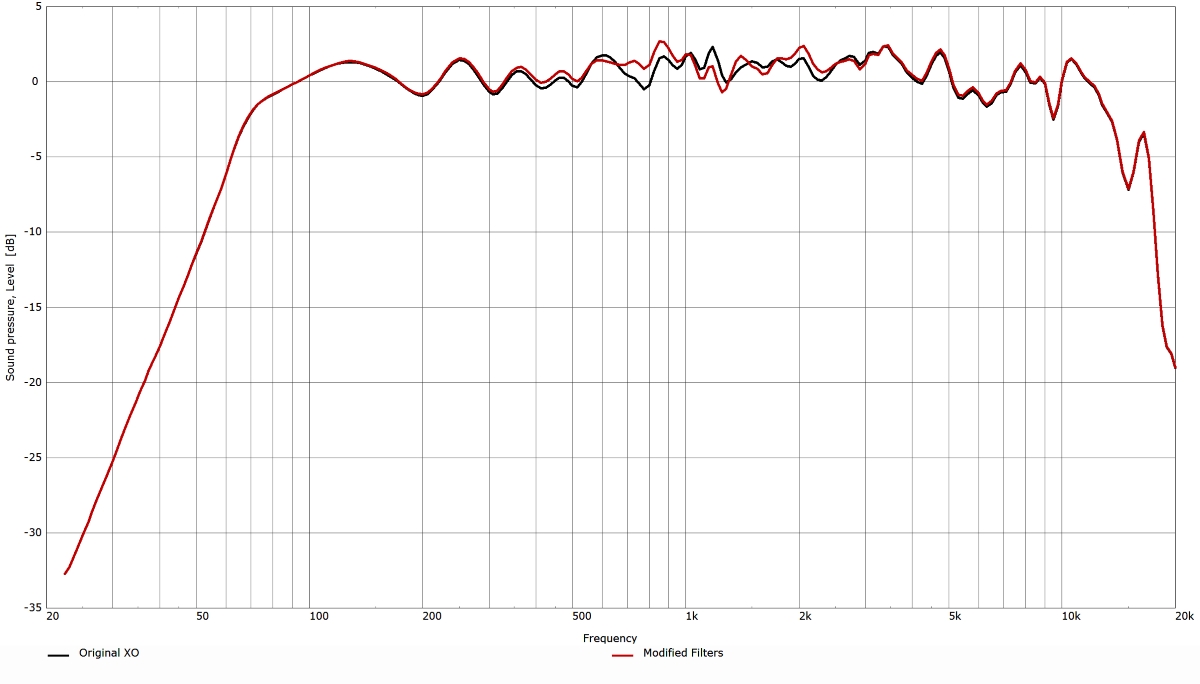
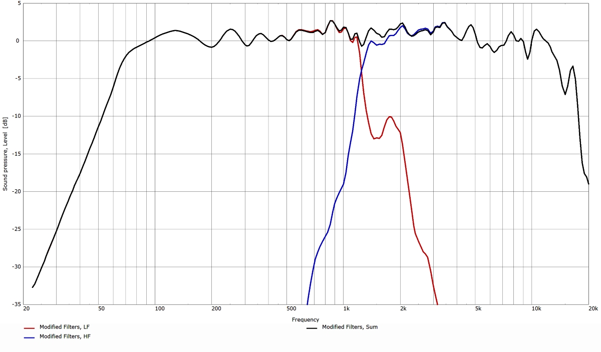
The on-axis frequency response of the LF and HF pass bands, along with the combined summation, using the modified filters are shown in Figure 6.

Compared to Figure 2 , the summation through the crossover region is good, however the level of the LF and HF pass bands is higher to get the same overall SPL though the crossover region. This is due to the change in the relative phase response between the LF and HF pass bands, which is required to achieve the more uniform vertical off-axis response.

A comparison of the on-axis responses using the original crossover and the modified filters (Figure 7) shows that there has been almost no change to the on-axis response. A comparison of the vertical directivity maps (Figure 4 and Figure 5) shows the off-axis response is now much more consistent, as well as being more similar to the on-axis response.