This will not be the case due to our vertically spaced sources.
Incidentally, all of the modeling was performed by and most of the graphs generated with SpeakerLab/GLL software from AFMG. It allows for some very nice investigation and optimization work to be carried out and displayed.
We have ideal text book sources so we will use fourth order Linkwitz-Riley low-pass and high-pass filters with a corner frequency of 1 kHz for our crossover.
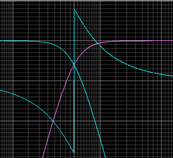
The on-axis summation of the sources in the far field with these filters is shown in Figure 4. This is exactly what we would expect. The low frequency level is +6 dB compared to the high frequency with a smooth transition in the crossover region.
This level change is because of the two woofers compared to the one horn (the point sources we are using each have identical output).

We also notice 360 degrees total phase shift due to the fourth-order filters. We get 90 degrees of phase shift for each filter order.
If we look at the off-axis response shown in Figure 5 we see that things are not quite so well behaved. There is considerable cancellation off-axis from 500 Hz up through the crossover region.

The directivity map has frequency plotted on one axis and the vertical radiation angle on the other axis. The output level is shown both as color variation and as elevation above the frequency-radiation angle plane.
All of the off-axis response data are normalized to the on-axis response. A slice through this surface at a given frequency will yield the polar response at that frequency.
Similarly, a slice through any radiation angle will yield the frequency response at that angle relative to the on-axis response.

For reference, polar plots at 500 Hz and 1 kHz are shown in Figure 6. Notice the deep nulls at +90 degrees and -90 degrees (straight up and down) in the 500 Hz polar and the same depressions in the directivity map (-20 dB green region).
Also, at 1 kHz the level drops quickly at off-axis angles, increases a bit, drops again and then increases back to full level. This is can be seen in the rippling of the directivity map. Compare this to the 1 kHz polar plot.