Voltage Variations—Make Up Your Mind
The particular number of 70.7 volts originally came about from the second way that constant-voltage distribution reduced costs:
Back in the late ‘40s, UL safety code specified that all voltages above 100 volts peak (“max open-circuit value”) created a “shock hazard,” and subsequently must be placed in conduit—expensive—bad.
Therefore working backward from a maximum of 100 volts peak (conduit not required), you get a maximum rms value of 70.7 volts (Vrms = 0.707 Vpeak). [It is common to see/hear/read “70.7 volts” shortened to just “70 volts”—it’s sloppy; it’s wrong; but it’s common—accept it.]
In Europe, and now in the U.S., 100 volts rms is popular. This allows use of even smaller wire. Some large U.S. installations have used as high as 210 volts rms, with wire runs of over one mile.
Remember: the higher the voltage, the lower the current, the smaller the cable, the longer the line. [For the very astute reader: The wire-gauge benefits of a reduction in current exceeds the power loss increases due to the higher impedance caused by the smaller wire, due to the current-squared nature of power.]
In some parts of the U.S. safety regulations regarding conduit use became stricter, forcing distributed systems to adopt a 25 volt rms standard. This saves conduit, but adds considerable copper cost (lower voltage = higher current = bigger wire), so its use is restricted to small installations.
Calculating Losses—Chasing Your Tail
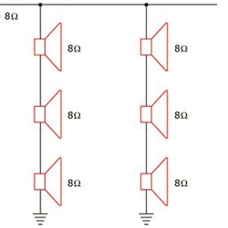
As previously stated, modern constant-voltage amplifiers either integrate the step-up transformer into the same chassis, or employ a high voltage design to direct-drive the line. Similarly, constant-voltage loudspeakers have the step-down transformers built-in as diagrammed in Figures 2 and 3.
The constant-voltage concept specifies that amplifiers and loudspeakers need only be rated in watts. For example, an amplifier is rated for so many watts output at 70.7 volts, and a loudspeaker is rated for so many watts input (producing a certain SPL). Designing a system becomes a relatively simple matter of selecting speakers that will achieve the target SPL (quieter zones use lower wattage speakers, or ones with taps, etc.), and then adding up the total to obtain the required amplifier power.
For example, say you need (10) 25 watt, (5) 50 watt and (15) 10 watt loudspeakers to create the coverage and loudness required. Adding this up says you need 650 watts of amplifier power—simple enough—but alas, life in audioland is never easy. Because of real-world losses, you will need about 1000 watts.
Figure 4 shows the losses associated with each transformer in the system (another vote for direct-drive), plus the very real problem of line-losses. Insertion loss is the term used to describe the power dissipated or lost due to heat and voltage-drops across the internal transformer wiring. This lost power often is referred to as I2R losses, since power (in watts) is current-squared (abbreviated I2) times the wire resistance, R.
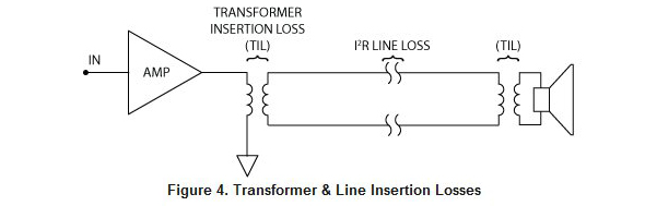
This same mechanism describes line-losses, since long lines add substantial total resistance and can be a significant source of power loss due to I2R effects. These losses occur physically as heat along the length of the wire.
You can go to a lot of trouble to calculate and/or measure each of these losses to determine exactly how much power is required [3], however there is a Catch-22 involved: Direct calculation turns out to be extremely difficult and unreliable due to the lack of published insertion loss information, thus measurement is the only truly reliable source of data.
The Catch-22 is that in order to measure it, you must wait until you have built it, but in order to build it, you must have your amplifiers, which you cannot order until you measure it, after you have built it!
The alternative is to apply a very seasoned rule of thumb: Use 1.5 times the value found by summing all of the loudspeaker powers. Thus for our example, 1.5 times 650 watts tells us we need around 975 watts.
Wire Size—How Big Is Big Enough?
Since the whole point of using constant-voltage distribution techniques is to optimize installation costs, proper wire sizing becomes a major factor. Due to wire resistance (usually expressed as ohms per foot, or meter) there can be a great deal of engineering involved to calculate the correct wire size.
The major factors considered are the maximum current flowing through the wire, the distance covered by the wire, and the resistance of the wire. The type of wire also must be selected. Generally, constant-voltage wiring consists of a twisted pair of solid or stranded conductors with or without a jacket.
For those who like to keep it simple, the job is relatively easy. For example, say the installation requires delivering 1000 watts to 100 loudspeakers. Calculating that 1000 watts at 70.7 volts is 14.14 amps, you then select a wire gauge that will carry 14.14 amps (plus some headroom for I2R wire losses) and wire up all 100 loudspeakers. This works, but it may be unnecessarily expensive and wasteful.
Really meticulous calculators make the job of selecting wire size a lot more interesting. For the above example, looked at another way, the task is not to deliver 1000 watts to 100 loudspeakers, but rather to distribute 10 watts each to 100 loudspeakers. These are different things. Wire size now becomes a function of the geometry involved.
For example, if all 100 loudspeakers are connected up daisy-chain fashion in a continuous line, then 14.14 amps flows to the first speaker where only 0.1414 amps are used to create the necessary 10 watts; from here 14.00 amps flows on to the next speaker where another 0.1414 amps are used; then 13.86 amps continues on to the next loudspeaker, and so on, until the final 0.1414 amps is delivered to the last speaker.
Well, obviously the wire size necessary to connect the last speaker doesn’t need to be rated for 14.14 amps. For this example, the fanatical installer would use a different wire size for each speaker, narrowing the gauge as he went. And the problem gets ever more complicated if the speakers are arranged in an array of, say, 10 x 10, for instance.
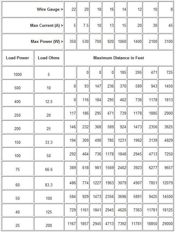
Luckily tables exist to make our lives easier. Some of the most useful appear in Giddings [3] as Tables 14-1 and Table 14-2 on pp. 332-333. These provide cable lengths and gauges for 0.5 dB and 1.5 dB power loss, along with power, ohms, and current info. Great book. Table 1 below reproduces much of Gidding’s Table 14-2 [4].
References
1. Langford-Smith, F., Ed. Radiotron Designer’s Handbook, 4th Ed. (RCA, 1953), p. 21.2.
2. Earley, Sheehan & Caloggero, Eds. National Electrical Code Handbook, 5th Ed. (NFPA, 1999).
3. See: Giddings, Phillip Audio System Design and Installation (Sams, 1990) for an excellent treatment of constant-voltage system designs criteria; also Davis, D. & C. Sound System Engineering, 2nd Ed. (Sams, 1987) provides a through treatment of the potential interface problems.
4. Reproduced by permission of the author and Howard W. Sams & Co.
Supplied by Rane. For more, visit the Rane Library.
Dennis Bohn is a principal partner and vice president of research & development at Rane Corporation. He holds BSEE and MSEE degrees from the University of California at Berkeley. Prior to Rane, he worked as engineering manager for Phase Linear Corporation and as audio application engineer at National Semiconductor Corporation. Bohn is a Fellow of the AES, holds two U.S. patents, is listed in Who’s Who In America and authored the entry on “Equalizers” for the McGraw-Hill Encyclopedia of Science & Technology, 7th edition.