Useful & Detrimental Reverberation
Reverberation is a very involved topic beyond our scope here, but it can roughly be subdivided in two categories: useful and detrimental. Useful reverberation consists of phenomena such as early reflections whereas detrimental reverberation consists of phenomena such as discrete echoes.
It would be extremely ill-advised to make EQ decisions based on echo-contaminated measurements since echoes don’t “un-equalize” the loudspeaker or sound system. Echoes are late arriving discrete copies of sounds, that originated at a source, which have become “un-fused” from the direct sound (first arrival).
If you’re dealing with echoes, re-aim the loudspeakers and work to keep their sound away from specular surfaces that reflect, which causes the echoes (prevention). The other option is to absorb the sonic energy upon impact when re-aiming is not an option (symptom treatment). EQ should only be used as a last resort when all other options have been exhausted, because EQ can’t differentiate between the very thing we’re trying to preserve: the mix, and the thing we’re trying to prevent: the echo (first, do no harm). If analyzers could somehow reject echoes, it would help prevent making poor EQ choices.
Time Blind
In the absence of noise, RMS- and vector-averaged transfer functions are expected to look the same when the delay locator is properly set; that’s to say, when measurement and reference signals are properly synchronized. Which raises the question: what happens if they’re not? In other words, what happens if the measurement signal arrives out of time?
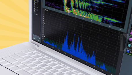
The finite linear impulse response (think of an oscilloscope) shown in the video in the upper plot of what is Figure 7 is also known as the “analysis window” whose duration is determined by the FFT-size and sample rate. In this example, the FFT-size is 16K (214 = 16384 samples) which at a sample rate of 96 kHz translates to a 171-milisecond-long window.
Signals that arrive in the center of the analysis window, while the “door” is ajar, are properly synchronized and arrive in time whereas signals which arrive outside the analysis window are out of time. How will this affect the transfer functions depending on the magnitude averaging type?
The RMS-averaged transfer function (blue) continues to look the same, even when the measurement signal arrives outside the analysis window, like echoes are known to do. This implies that RMS averaging can’t tell direct sound from indirect sound and is time blind! Like noise, reverberant energy can only add to the RMS-averaged transfer function (blue) and make it rise whether it’s on time or not.
Remarkably, the vector-averaged transfer function drops proportionally as the measurement signal moves towards the edge of the analysis window. By the time the measurement signal arrives outside the analysis window (late by 85 ms or more) it has been attenuated by at least 10 dB for the current number of averages. Increasing the number of (vector) averages will attenuate the signal even further. It’s like “virtual” absorption has been applied which attenuates late arriving signals such as echoes (unlike RMS averaging, which is time blind).
So how late does a signal have to be to constitute an echo?
Tap Delay
Classic literature typically states single values for the entire audible band, e.g., 60 ms, which is a vocal-centric answer. However, there’s no such thing as a single-time-fits-all-frequencies delay. Sixty milliseconds equal 0.6 cycles when you’re 10 Hz, 6 cycles when you’re 100 Hz, 60 cycles when you’re 1 kHz, and 600 cycles when you’re 10 kHz. After 60 ms, certain (lower) frequencies have barely finished, or are still in the process of finishing, their first complete revolution, how could they possibly have become echoic?
A conservative estimate but more realistic delay (again, for reasons beyond the scope of this article) is 24 cycles, which is also frequency dependent. Twenty-four cycles equal 240 ms at 100 Hz, 24 ms at 1 kHz, and only 2.4 ms at 10 kHz! It’s clearly not the same time for all frequencies. When we pursue the idea of a sole time delay for all frequencies, we’re doing a tap delay – which is a “rhythmic” echo – whereas real echoes are two or more discrete instances of the same signal that have become un-fused, and where the time gap is frequency dependent.
So, while vector-averaging is capable of attenuating echoes which arrive outside the analysis window, clearly a single fixed analysis (time) window won’t suffice.
Multiple (Analysis) Time Windows
Modern analyzers use multiple time windows for the entire audible band instead of a single fixed window. This allows them to hit two birds with one stone. First, multiple windows produce a quasi-logarithmic frequency resolution or fixed points per octave (FPPO), unlike a fixed window where resolution is proportional to frequency. In order to achieve FPPO, short time windows (typically 2.5 ms) are used for high frequencies, and as we go down in frequency, the window duration is increased exponentially to about 1 second for the lowest frequencies.
This brings us to the second important advantage of multiple windows, which is that high-frequency echoes will be rejected much sooner than low-frequency echoes, provided we resort to vector-averaging and properly set the delay locator. This gives vector-averaging the capability to capture and preserve useful reverberation such as (stable) early reflections that strongly affect tonality, and arrive inside the analysis time windows, while rejecting detrimental reverberation such as echoes which arrive outside the analysis time windows. To RMS averaging it’s all the same…
It would be really convenient if there was one more metric that could increase our confidence and keep us from making poor EQ decisions.
Coherence
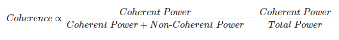
Coherence is a statistic metric that’s proportional to the ratio of coherent signal power to coherent plus non-coherent signal power (which is the total signal power). It describes the fraction of a system’s total output signal power that is linearly dependent on its input signal power (Equation 1).
In the absence of non-coherent signals, coherence is expected to have a value of 1, or 100 percent. In the absence of coherent signals, coherence is expected to have a value of 0, or 0 percent. It’s a “lump” indicator because non-coherent signals come in many flavors.
Since coherence is always computed vectorially, it’s susceptible to phenomena such as noise, late-arriving energy outside the analysis windows (echoes), and even distortion. What it won’t do is tell us which is which. For that, we need an analyzer that’s not the software. The software is just a tool, like an army knife. We users are the actual analyzers (thank you Jamie Anderson) and it’s up to us to determine the nature of non-coherent power…
Putting It Together
High-coherence data is actionable data. Figure 8 provides an example of an extremely lousy measurement that makes for a good example. As of version 8.4.1, Rational Acoustics Smaart software now provides the option to display squared coherence like Meyer Sound SIM, which is very convenient.
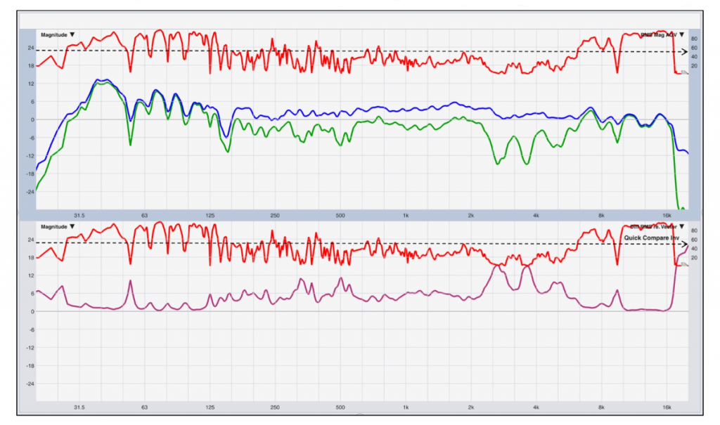
If we look at Equation 1, we should be able to appreciate that one part coherent power and one part non-coherent power equals half (or 50 percent) coherence, or a 0 dB coherent-to-non-coherent power ratio. In other words, 50 percent is the break-even point which is indicated with the black dashed line in both plots.
RMS- and vector-averaged transfer functions are expected to be near identical when coherent power exceeds non-coherent power by 10 dB, independent of the flavor of non-coherent power. Since coherence deals with signal power, you should apply the 10log10 rule that informs us that +10 dB equals a factor x10. Therefore, 10 parts coherent power against one-part non-coherent power equal 10/11 (Equation 1) or 91 percent coherence.
When coherence equals 91 percent or more, notice that both transfer functions in the upper plot are in good agreement. However, once that condition is no longer met, the traces start to differ substantially. By how much exactly can be viewed in the bottom plot, where we see the difference with help of “Quick Compare.”