RMS Averaging
Root-Mean-Square (RMS) averaging is effectively signal power averaging. From Ohm’s law we can derive that power is proportional to squared amplitude values, and power is a scalar which is a quantity represented by a sole value that describes its magnitude. Meanwhile, the squaring operation in RMS robs us of the sign (and signs matter) leaving us with only positive values.
“Whether you owe me money or I owe you money, the difference is only a minus sign.” – Walter Lewin, former MIT physics professor
When dealing with scalars, there’s no direction that makes RMS averaging time blind, as we’re about to discover.
Vector Averaging
A vector (think of an arrow) is a quantity that’s represented by two values that describe the vector’s magnitude (the length of the arrow) and its direction (which way is the arrow pointing). Noise at a constant level can be represented by a vector whose magnitude remains constant over time, but whose direction changes randomly over time (Figure 4). When multiple vectors of constant magnitude, whose direction is random (random phase angle) are averaged, the mean magnitude collapses to zero as the number of averages is increased.
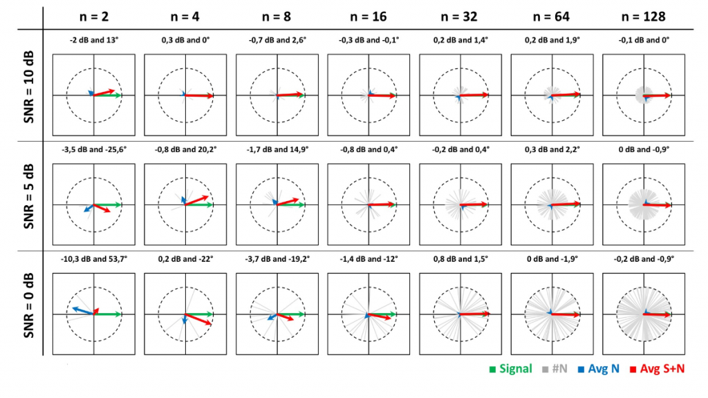
However, our excitation signal, when represented by a vector, preserves direction as well as magnitude over time. When averaged, the mean magnitude and direction are expected to be identical to the average’s constituent components (our excitation signal). Notice that in Figure 4, both magnitude and direction for signal-plus-noise approach those of signal, which is what we’re ultimately after, as SNR or the number of averages is increased.
As with our hearing sense and brain in the crowded bar, vector averaging features the ability to progressively reject noise with increasing averaging. Further, having a direction descriptor in addition to magnitude (unlike the scalar), makes vectors subject to phase angles and inherently time.
When do RMS and vector averaging produce identical transfer functions? Only when:
1) Measurement and reference signals are properly synchronized (delay locator).
2) There’s little to no contamination by non-coherent signals, i.e., ample SNR and D/R.
Figure 5 shows that as long as there’s ample SNR, i.e., 10 dB or more, as seen at 125 Hz and below, RMS- and vector-averaged transfer functions are in good agreement. But, with 0 dB of SNR or less, as seen at 1 kHz and above, noise determines the appearance of the RMS-averaged transfer function (blue) and no amount of averaging will change that.
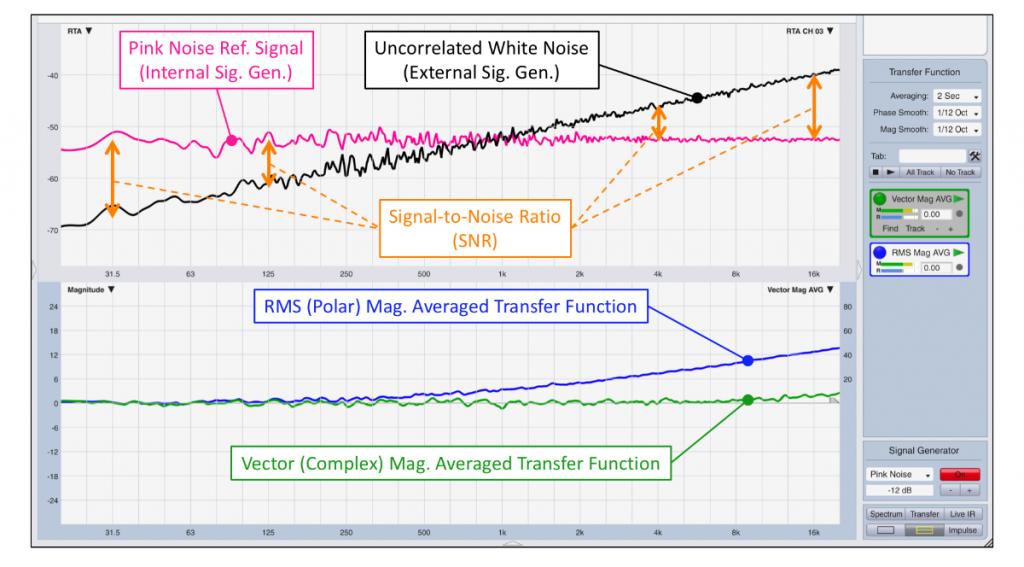
Are you convinced that an audience is always 10 dB less loud than the sound system during songs? Notice that the vector-averaged transfer function (green), even for negative signal-to-noise ratios (SNR less than zero), remains virtually unaffected with help of a modest amount of averaging.
Hostile Environment
In the real world, comb filtering is inevitable, and its frequency response ripple is a function of the relative level offset between the comb filter’s constituent signal copies.
In the absence of noise, both RMS- (blue) and vector-averaged (green) transfer functions in Figure 6 are indeed identical. When SNR is reduced to 20 dB (black line spectrum in RTA plot), with respect to the signal’s spectral peaks (pink line spectrum in the RTA plot), appearances change. (Editor’s Note: There’s a video embedded later in this article — Figure 7 — that adds further clarity to Figure 6 and the discussion.)
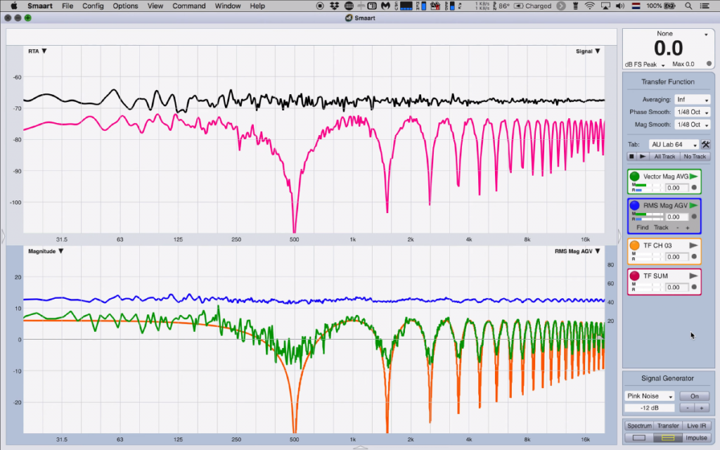
\Notice that the cancels (valleys) of the RMS-averaged transfer function (blue) rose, which is also true for the vector-averaged transfer function (green), but to a much lesser extent as we can tell from looking at the orange trace underneath, which is the original comb filter in the absence of noise. The transfer function peaks for both types of averaging are in good agreement.
When SNR is reduced to 10 dB, the blue valleys rise substantially, which reveals a serious weakness of RMS averaging which is that its incapable of distinguishing noise from signal. Signal (pink) has been destroyed at certain frequencies due to destructive interaction and all that’s left at those frequencies is residual background noise (black) that “fills” these cancels (valleys).
Regardless, this uncorrelated contamination makes the RMS-averaged transfer function look different. The vector-averaged transfer function (green), with help of a slight increase in averaging, remains in much better agreement with the orange reference trace. The transfer function peaks for both types of averaging are still in good agreement with 10 dB of SNR.
When SNR is reduced to 5 dB, the frequency response ripple for the RMS-averaged transfer function (blue) is about 6 dB. It appears as if we’re in an anechoic room (refer back to Figure 1), whereas the vector-averaged transfer-function (green) persists and shows us the real deal; that is to say, the actual degree of interaction which we can tell from the green ripple that has not been obfuscated by noise.
Also, with this little SNR (5 dB), the transfer function peaks for both types of averaging are no longer in good agreement. For all frequencies, the RMS-averaged transfer function (blue) rose which is the limitation of RMS averaging where signs have been lost. As SNR is reduced, RMS-averaged transfer functions can only go up.
When SNR is reduced to 0 dB, both transfer functions look completely different. The vector-averaged transfer function (green) persists and continues to show how severely compromised the system is (strong ripple) unlike the RMS-averaged transfer function (blue) where the first cancel (valley) that is 1-octave wide (11 percent of the audible spectrum) has been filled to the top with noise (which also goes for the remaining cancels).
Finally, when SNR is reduced to -6 dB and noise is now actually louder than signal, the blue RMS-averaged transfer function suggests there’s no (destructive) interaction whatsoever, whereas the green vector-averaged transfer function persists. Under such extreme conditions, one can even set the averager to infinity (accumulate) in which case it continues to average for as long as the measurement is running, improving SNR artificially as time passes by. How long should we average? Until there’s no apparent change in the data? Why wait longer without getting anything in return?
By now, I hope you can appreciate how (background) noise can really mess with the appearance of transfer functions depending on how the analyzer is set up, and EQ decisions should be made with scrutiny. However, noise is just one subset of a larger family of non-coherent signals.
Real-world measurements of loudspeakers and sound systems will be contaminated with non-coherent signals; that is to say, uncorrelated signals that are not caused exclusively by a system’s input signal (causality), or correlated signals that are no longer linearly dependent on the system’s input signal. Non-coherent signals come in many flavors such as noise (like our audience), late arriving energy (reverberation) outside the analysis window and distortion.