
Cylindrical waves lose only 3 dB rather than 6 dB per distance doubling, making them very marketable. After all, they cut the expected propagation losses known of point sources in half!
And as a consequence, ever since the advent of modern line arrays – in the early 1990s – many subsequent claims about cylindrical waves may have been exaggerated. So much so that newcomers, at the time of writing, continue to get indoctrinated with a firm belief that line arrays simply work by virtue of cylindrical waves without questioning: a) when, i.e., for what frequencies, and b) where, i.e., up in the air (above the audience) or in the audience plane (across the audience), or both.
This article explores whether or not real-world line arrays exhibit expected line source behavior. And more importantly, when and where in space such behavior is observed. Up in the air (above the audience) or across the audience – in the audience plane – or both (Figure 1)? The distinctions will not be trivial.
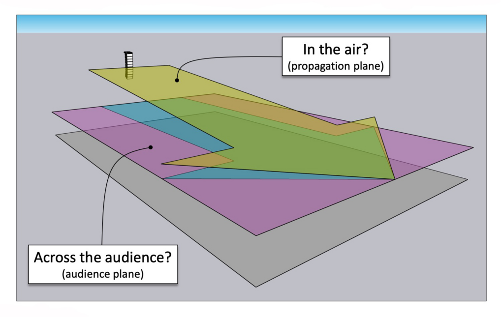
This article will also question if referencing “cylindrical waves” – in the context of line arrays – has been hyped for its marketability. And whether or not it is the most concise term for describing a line array’s unique behavior across the audience – i.e., in the audience plane – rather than up in the air (above the audience).
Invariably, newcomers and seasoned veterans alike ask about cylindrical waves when discussing line arrays. During a seminar in Switzerland a couple of years ago, I found myself very much annoyed by learning that (future) audio professionals – already in school – continue to get indoctrinated with a firm belief that line arrays simply work by virtue of cylindrical waves without questioning when and where in space the behavior may or may not occur.
As far as the author can tell, the behavior of loudspeaker line arrays, both curved as well as straight, was first described by Harry F. Olson in his seminal book “Elements of Acoustical Engineering” all the way back in 1940.
As we speak, line arrays have been commercially available for three decades. Suffice to say, the theory surrounding line arrays is both mature and well known. And yet, this indiscriminate, oversimplified notion of “cylindrical waves” continues to persist. And to a large extent under the influence of marketing.
Point Source Or Line Source?
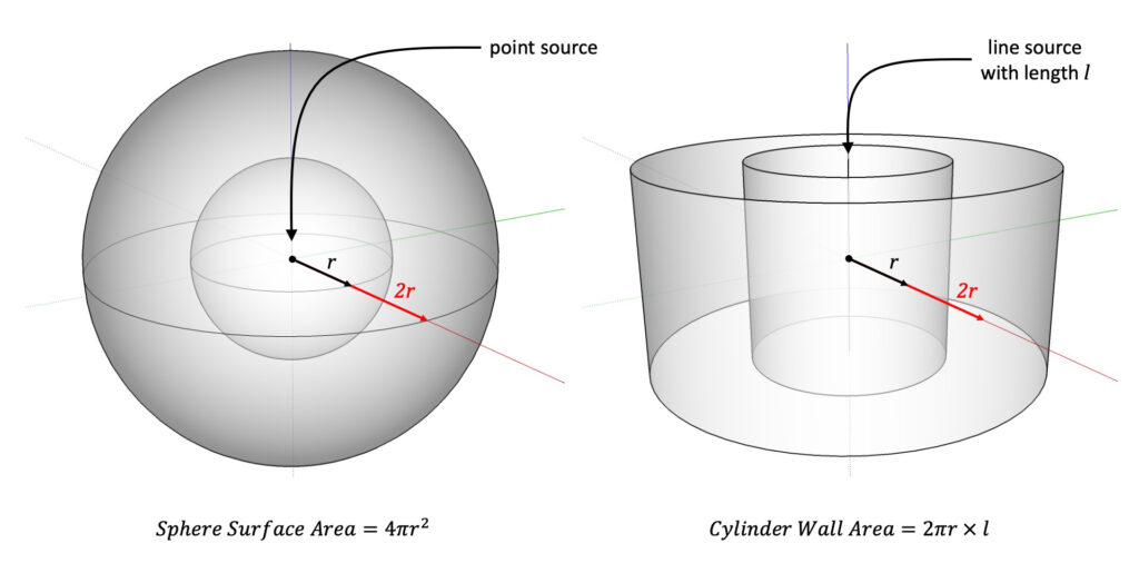
A point source emits a wave that expands spherically in two dimensions. The surface area of a sphere equals 4πr2 (Figure 2) and expands at a rate proportional to r2. When sound travels twice as far, the sphere’s radius is doubled. The finite amount of radiated energy spreads uniformly over four times the surface area. As such, sound level loss over distance adheres to the 1/r2 dependency at a rate of -6 dB per distance doubling. This is known as the inverse square law (ISL).
An ideal continuous line source emits a wave – across its entire length – that expands cylindrically in only one dimension. The surface area of a cylinder wall (whose height matches the length of the line source) equals 2πr×l and expands at a rate proportional to r.
When sound travels twice as far, the cylinder’s radius is doubled as well. However, the finite amount of radiated energy spreads uniformly over only twice rather than four times the surface area. As such, sound level loss over distance adheres to the 1/r dependency at a rate of only -3 dB per distance doubling.
Whether or not the latter behavior is actually observed for practical systems remains to be seen. And when it occurs, for what frequencies, and where in space does it happen? (Again: up in the air, above the audience, or across the audience, in the audience plane – or both?) Let’s start by looking at what happens – in the air – along an array’s central propagation axis.
Above The Audience
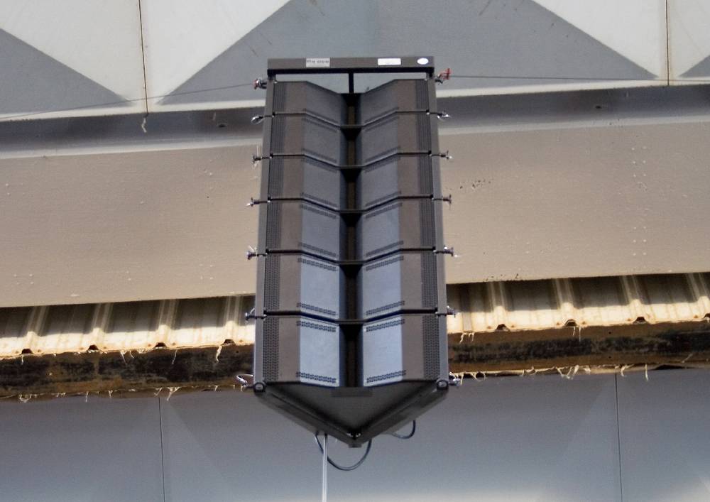
The following examples were inspired by an approach published in a loudspeaker manufacturer’s technical report from the early 2000s, in which they modeled 100 one-inch pistons, complete with pistonic behavior, whose centers are spaced one inch apart – effectively constructing a straight 2.5-meter tall column loudspeaker.
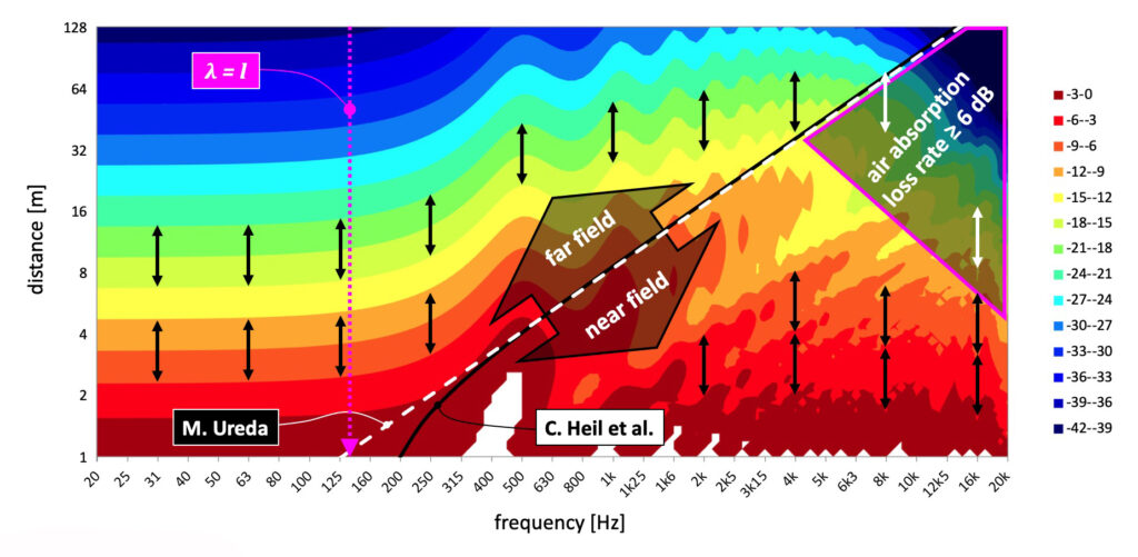
Figure 3 shows the axial response—without air absorption—as a function of distance relative to one meter. Where distance is shown deliberately on a logarithmic scale, such that the length of each double-headed arrow corresponds with a doubling in distance. With 3 dB per color division, two color divisions per double-headed arrow correspond with a 6 dB loss, i.e., point source behavior, whereas one color division per double-headed arrow suggests line source behavior with a loss of only 3 dB per distance doubling.
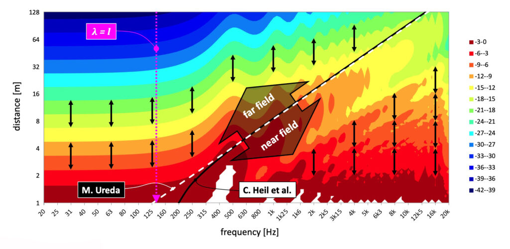
For all frequencies whose wavelength exceeds the array length where λ>l
(i.e., 344 ms ÷ 2.54 m ≈ 135 Hz or less) – independent of the observation distance – we exclusively see point source behavior with two color divisions per distance doubling. The array is too short to introduce line source behavior.
Whereas the sound level loss rates for the remaining frequencies – above 135 Hz – can be roughly divided into two zones. One zone that diminishes with increasing frequency, where we continue to observe two color divisions per distance doubling (point source behavior) known as the “far field.” And another zone that expands with increasing frequency, where we observe one color division per distance doubling (line source behavior) known as the “near field.”
The initial separation between consecutive contours (that separate the colors) is denser for lower frequencies and sparser for higher frequencies. Which means that the latter have been subject to a – decelerated – loss rate of less than 6 dB per distance doubling.
In exchange, these higher frequencies get to “throw” farther. However, with increasing observation distance, the separation between consecutive contours for higher frequencies gets denser until you once more see two color divisions (rather than one) per distance doubling. And linesource behavior reverted to point source behavior.
The axial transition distance (also known as border distance) from the near field into the far field – for straight arrays – can be calculated (but not limited to) in various ways.
According to Christian Heil, et al in 1992:
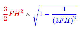
where F is frequency in kilohertz, and H is the height of the line source in meters.
With increasing frequency, the second term of previous equation tends to one, leaving only the first term that can be re-written as:
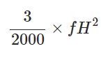
where f is frequency in hertz and H is the height of the line source in meters.
And according to Mark Ureda in 2001:
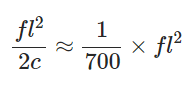
where f is frequency in hertz, l is the length of the line source in meters, and c is the soundspeed in meters per second (m/s).
Notice that the fractions in the last two equations are functionally the same, which explains why both transition lines in Figure 3 are in good agreement. Regardless, in either case, the near- to far-field transition for straight finite-length arrays is a moving target that is proportional to frequency and array length squared. Notice that the transition distance doubles with each octave, but quadruples when an array is made twice as long.
Consequently, an everlasting near field – for all frequencies – can only be achieved by infinitely long arrays. (When was the last time you worked with an infinitely long line array?) Whereas real arrays will always be a hybrid solution featuring both point source and line source behavior.
Once More With Air Absorption
So far, for straight arrays – without air absorption – we have indeed observed initial line source behavior confined to a) higher frequencies, and b) up to maximum distances. In reality however, high-frequency air absorption by the propagation medium is unavoidable.
Figure 4 shows the same configuration, but this time with air absorption. Notice that air absorption causes the very‑high frequencies’ sound‑level loss‑rates to collapse with increasing observation‑distance.
For very high frequencies, propagation through the medium has accelerated the initial 3 dB per doubling distance loss rate (associated with line source behavior) to the point that it once more becomes 6 dB per doubling distance and even worse.
As a consequence, and contrary to the trend observed at mid-high frequencies, the resulting trend at very high frequencies has more in common with the point source behavior observed at low frequencies (where λ > l). Air absorption has penalized the “throw” of the very high frequencies.
Mid high frequencies, unaffected by air absorption while still exhibiting initial line source behavior, now get to “throw” the farthest. When left unchecked, they will cause the much dreaded nasalquality, edgy, proverbial “ice pick in the forehead” that’s further exacerbated by zero degree interelement splay angles (remember, the array has been straight so far). After all, tonality over distance is only preserved when all frequencies drop at the same rate, which clearly is not the case.
Once More With Constant Curvature
Rather than continuing with a straight array, let’s introduce some mechanical articulation to the 100 x 1-inch piston array. Figure 5 shows four constant curvature arrays whose total array splay ranges from 10 to 90 degrees by virtue of identical (albeit different) inter-element splays.
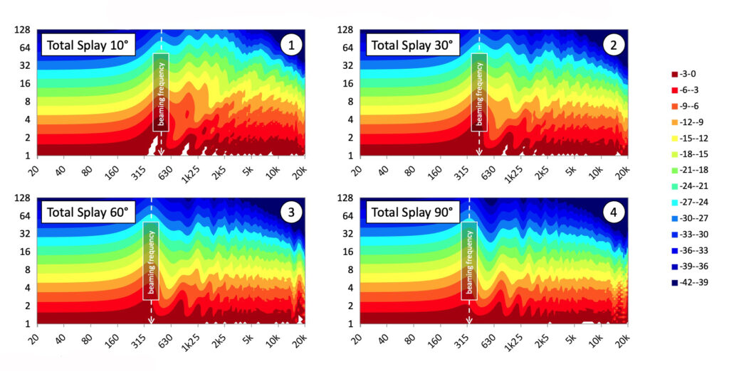
Notice that by increasing total array splay, the initial net loss rates (associated with line source behavior) collapse even further with decreasing frequency, making mechanical articulation, besides frequency and array length, the third variable that determines “throw.”
Regardless, for this specific 2.5-meter tall array, up in the air – not to be mistaken for across the audience – while taking all aggravating conditions into consideration, including (but not limited to) air absorption and array curvature, it’s pretty much game-over beyond eight to 16 meters. With increasing observation distance, the array (for most frequencies) clearly gravitates towards point source rather than line source behavior.
The remaining (least decelerated) low-mid frequencies now get to “throw” the farthest. These are closely related with the “beaming frequency” where various DSP-based beam steering techniques, beyond the scope of this article, come in. (Please refer to my article “Pick Your Battles” on ProSoundWeb for more information on this topic.)
Nevertheless, “throw” can be increased or decreased – within reason – by virtue of array curvature (albeit for a limited range of frequencies). Notice in Figure 5 there’s no significant change at lower frequencies (where λ>l), regardless of the array curvature.
In The Audience
Up until now, we’ve been solely focusing on what happens in the air along the array’s central propagation axis, which is not where the audience typically resides in space. Figure 6 shows an actual 100 element array covering a standing audience up to a depth of 25 meters.
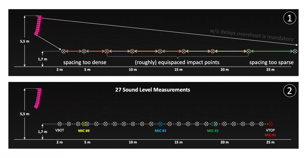
The range ratio is a little over 8:1, i.e., audience members in the back are 20 × log10(8) = 18 dB more distant than audience members in the front. It will take at least 12 dB of amplitude steering, by virtue of mechanical articulation, to reduce the HF level drop across the entire audience to 6 dB or less, rather than 18 dB.
When the inter-element splay angles are set inversely proportional to distance, such that:

for some constant k where α is the interelement splay angle in radians, and d a single element’s throw distance up to its impact point (where the axial sound for a single element touches down in the audience). Then the separation between impact points ends up being roughly the same (Figure 6) which automatically results in the classic J-shaped array with tapered splays (less splay in the top of the array and more in the bottom).
It is intuitively pleasing to see the splay ratio (ratio of smallest and largest inter-element splay angles) reflect the range ratio. With, e.g., one degree in the top and a range ratio of 8:1, one would expect at least eight degrees or more in the bottom.
Small splays overlap adjacent elements, enabling them to throw high frequencies farther in a team effort. Whereas large splays effectively constitute a solo effort – without overlap – where high frequencies throw shorter distances. At the audience start, where audience members are 18 dB closer, the combined HF horsepower of all 10 loudspeakers is not required. The bottom loudspeaker alone will suffice. The other way around (a single loudspeaker for the back of the audience), not so much.
Meanwhile, beam narrowing, by virtue of array length (phase steering), which is a different mechanism altogether beyond the scope of this article, takes care of the lower frequencies where the loudspeakers become increasingly more omnidirectional and no longer respond to interelement splay angles.
Let’s see whether or not the mechanical articulation of this array achieved a 6 dB rather than 18 dB drop in level across the entire audience, i.e., 12 dB of steering.
A-Weighted Levels
Figure 7 shows the relative A-weighted sound level, according to the prediction software, of the (anechoic) direct sound – without air absorption – at the 27 measurement positions indicated in the bottom plot of Figure 6.
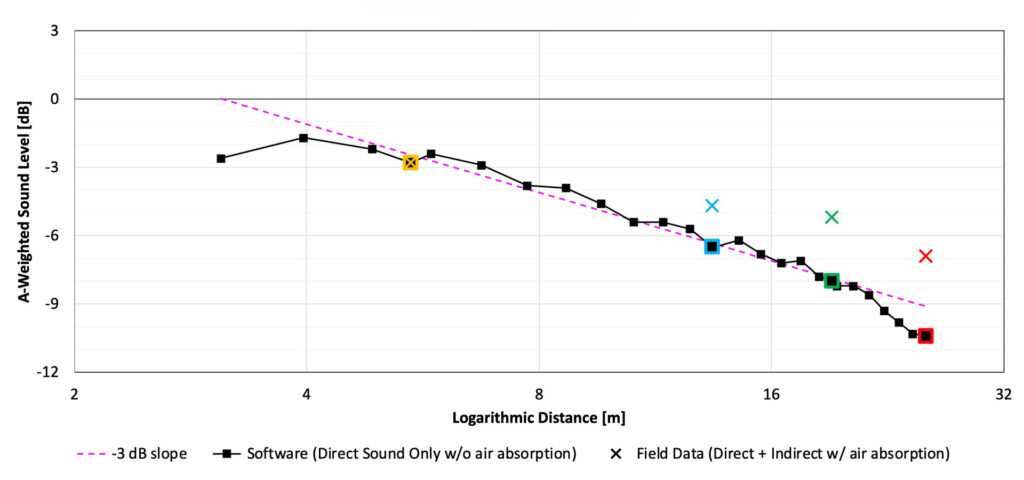
A-weighting is effectively a high-pass filter that rejects low frequencies. Measuring nearly 2.3 meters in length, this array will not exhibit line source behavior below 150 Hz. Therefore, to detect line source-like behavior, it makes sense to resort to A-weighting that only admits those frequencies where line source-like behavior is expected for an array of this length.
According to the prediction software, the expected level drop across the entire audience slightly exceeds 6 dBm which does not come as a surprise. In reality, the particular rigging hardware dictates the available splay settings and determines whether or not you will get to perfectly equi-separate the impact points.
Look at the top plot in Figure 6 and you’ll see that the impact point separation in the front is a little too dense and therefore too loud, and vice versa in the back of the audience, i.e., too sparse and therefore too soft. Further, I wouldn’t have minded another meter of trim height to raise the array in exchange for a slightly more favorable range ratio. (Welcome to the real world.)
Nevertheless, when the results are plotted on a logarithmic scale, a clear trend is visible. For the frequency range of interest, the sound level across the audience, i.e., in the audience plane – not up in the air above it – indeed drops at a rate of 3 dB per doubling distance, reminiscent of cylindrical waves. Does that mean marketing was right all along?
Pseudo-Cylindrical Behavior
Although exhibiting cylindrical behavior, it should be noted that the structure of the sound field has cylindrical effects on the audience only. The propagation through the air is still somehow in between cylindrical and spherical. For this reason, we will term the sound field radiated by a variable curvature line source as pseudo-cylindrical. – Urban et al (2001).
The term “pseudo-cylindrical” rather than just “cylindrical” is indeed a much more concise description of the observed behavior in Figure 7. And it correctly conveys a line array’s principal value proposition. While the loss-rate (for higher frequencies) across the audience may be reminiscent of cylindrical waves, regardless of what happens up in the air above the audience, no cylindrical waves propagate along the audience plane.
From what the author can tell, science has always been very clear on these very important distinctions. You now get to decide whether marketing did so too…
References
Elements of Acoustical Engineering Harry F. Olson (1940) ISBN-13: 9781376156539
Sound Fields Radiated by Multiple Sound Sources Arrays by C. Heil and M. Urban (1992) aes.org/e-lib
Line Arrays: Theory and Applications by Mark S. Ureda (2001) aes.org/e-lib
Wavefront Sculpture Technology by M. Urban, C. Heil, and P. Bauman (2001) aes.org/e-lib
Line Arrays: Theory, Fact and Myth by Meyer Sound (2002)