The impulse response, or simply IR, remains an abstract concept to many. But if we think of the impulse response literally as an audio track in a digital audio workstation (DAW) like Pro Tools, Logic or Reaper, it might bring welcome clarity.

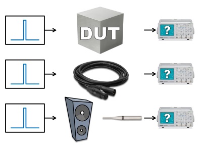
Let’s start with Bob McCarthy’s excellent explanation. The impulse response describes the answer to a hypothetical question: “What would this Device Under Test (DUT) look like on an oscilloscope when driven with an (im)pulse?” (Figure 1)

An oscilloscope displays audible sound as alternating current (AC) with positive and negative polarity where the ideal pulse (known as a Dirac pulse) would look like an instantaneous rise followed immediately by a fall without overshoot. It contains every audible frequency, lasting for exactly one cycle, starting at the same time and level.

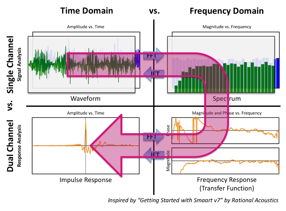
Dual-channel fast Fourier transform (FFT) analyzers can obtain an IR either directly or compute it as a second-generation transfer function from the frequency domain by means of the inverse Fourier transform (Figure 2).

This allows us to calculate the IR mathematically rather than having to fire an actual starting pistol, popping a balloon or clapping our hands. Time and frequency domain are reciprocal. They’re joined at the hip like two sides of the same coin. It’s exactly the same story told from different points of view.

If we introduce such a transient signal, e.g., a snare drum hit, into a microphone cable (a near-perfect conduit for our application), we expect it to come out at the other end instantaneously without any meaningful changes in time and/or level (Figure 1, Example 2).

But what happens if we introduce a pulse into a DUT exhibiting a gratuitous amount of phase shift like a loudspeaker or, in this instance, a subwoofer (Figure 1, Example 3)?

Figure 3 shows a DAW (Reaper) with three tracks. Track 1 contains the IR of a microphone cable and Track 2 the IR of a typical vented subwoofer with direct radiator(s) whose level has been normalized solely for visual purposes. Band-limiting a loudspeaker, like a subwoofer, reduces the amplitude of its IR which makes the waveform hard to see, particularly on the linear amplitude scale of a DAW or oscilloscope.

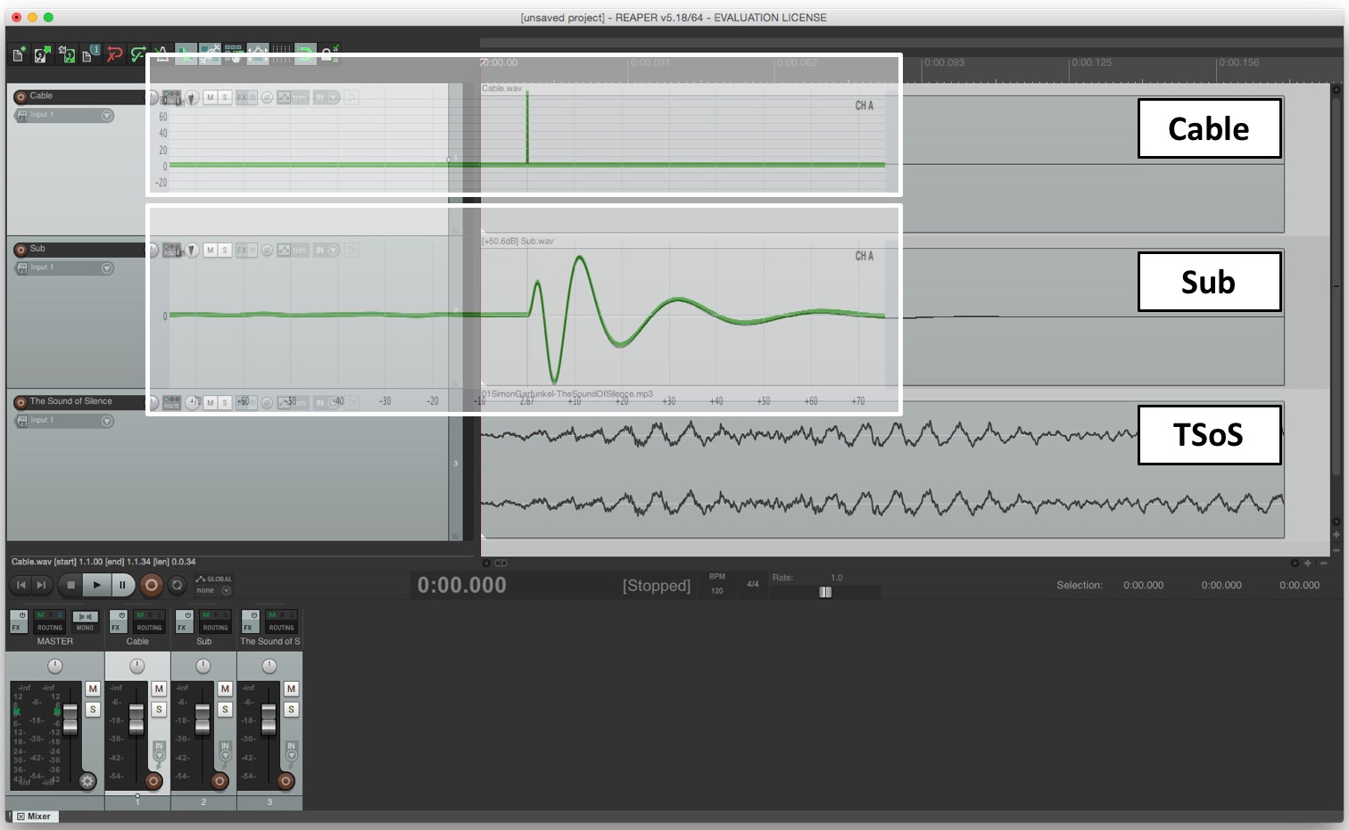
I’ve deliberately delayed both responses by 10 milliseconds (ms) so that their waveforms don’t appear directly at the beginning of their respective tracks. Track 3 shows an arbitrary fragment of “The Sound of Silence” by Simon and Garfunkel (pun intended) to emphasize the waveform concept.

I’ve superimposed these very same IRs, as observed in an analyzer, on top of Tracks 1 and 2, respectively. When we conduct transfer function analysis, we use internal delay to synchronize the two channels, thereby compensating for propagation delay (latency and/or time of flight). Notice here that this practice acts like the actual playback position in a DAW.

If we scrub through the pulse in our microphone cable (Track 1) all audible frequencies will be heard instantaneously at the peak, i.e., a single-sample event. By contrast, the inherent phase shift of our subwoofer (Track 2) has stretched the pulse out over time and scrubbing through its track will typically let us hear only a single subwoofer frequency at a time. It’s like sliding down the neck of a fretless bass guitar from high to low.