
Here we lay the foundation. We’ll look at analog to digital conversion, and we’ll look at the spectrum of the resulting digital signal. We’ll use that knowledge to help understand the conversion process back to analog.
Though we can build real-world converters that work as described, we’re not building practical converters here; we’re interested in the mathematical concepts involved and their relationships to digital signal processing.
Analog To Digital Conversion
The sampling theorem says that we can describe, uniquely, a continuous (analog) signal with evenly-spaced discrete (digital) samples, as long as the sampling rate is greater than twice the highest frequency component in the continuous signal. To ensure that we don’t violate that condition, we preface the analog to digital conversion with a low pass filter, set to pass frequencies below half the sample rate, and block those above:

The sampling process—basically taking repeated measurements as a fixed interval—can be viewed in a number of ways; here’s one that can help us understand some important aspects of sampling:
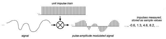
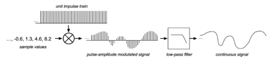
The input signal, after filtering to ensure our bandwidth condition, is modulated (multiplied) by a pulse train of unit amplitude. The result is a pulse-amplitude modulated signal. We measure the height of each modulated pulse, and store the numerical values as our samples.
The Spectrum Of A Sampled Signal
While our original signal can be anything, we must limit the frequency spectrum of the signal we sample to half the sampling rate—again, we ensure this condition by placing a low-pass filter before the sampling stage. So, we can represent the spectral limits of the signal by showing the response curve of the low-pass filter:
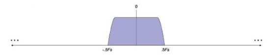
Here we’re showing positive and negative frequencies, in order to make the following more obvious.
The spectrum of the impulse train we’re using to multiply the input signal looks like this:
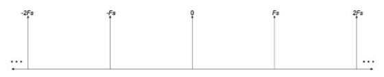
That is, the spectrum of an impulse train in time is an impulse train in frequency.In the time domain, the impulses are spaced at multiples of the sampling period, and in the frequency domain at multiples of the sampling frequency.
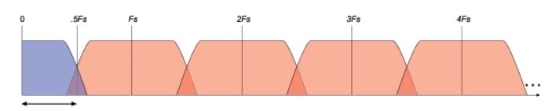
The result of the multiplication in the time domain is a convolution in the frequency domain—the result in the frequency domain is that we have spectral reflections of the original signal, centered on multiples of the sampling rate:
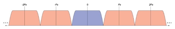
We don’t mind the reflections, since they stay out of the way of the signal band we care about, but if we had used a poorer low-pass filter or set its frequency too high, the reflections would overlap into the band we’re interested in—this is called aliasing (from here on we’ll look at the positive frequencies only, to save space, noting that the negative side is just a reflection):
A consequence of aliasing is that frequencies that exceed half the sample rate reflect back into our band of interest. For instance, a sine wave that sweeps in frequency above half the sample rate will seem to reverse and turn back down. High harmonics that cross over will be inverted, imparting an inharmonic tone to the sound. Once we let this happen, there is no way to tell the good from the bad, so we must minimize aliasing by using acceptable filters.
Now that we understand what we’ve done to the signal by sampling it, we can look at the process of converting the signal back to a continuous signal.
Digital To Analog Conversion
To convert from samples to the continuous domain, we perform what is pretty much the inverse process. In principal, we first turn the numbers into a pulse-amplitude modulated signal. This signal has the information we need, but carries some extra that we don’t want—images of our signal, aliased copies that appear at multiples of the sample rate. So, we strip off the high-frequency clones with a low-pass filter. Effectively, this smooths the pulse train into the signal we desire.
Note that the digital to analog conversion is similar to our analog to digital conversion, almost in reverse, except that in the case of converting from analog, the low-pass filter is precautionary—to guarantee we limit the bandwidth to avoid aliasing—while in the conversion from digital, the filter plays an integral role in reconstructing the signal. For that reason, the latter is often called the reconstruction filter.
Read and comment on the original article here.
Nigel Redmon is a musician, electrical and software engineer, and independent developer, specializing in digital audio signal processing applications. He has developed products for Line 6, Equator Audio, Alesis, Oberheim, and others.