Specular reflections can make a shamble of analyzer traces, which complicates data interpretation and sets the table for poor EQ choices. Windowing or gating in an attempt to rid ourselves of those pesky late arriving reflections reduces the “jaggedness” in our traces and thereby the need for excessive smoothing.

That said, modern analyzers typically already apply windowing under‑the‑hood in such a way that useful (stable, early) reflections are preserved while detrimental reflections (echoes) are rejected. While additional user‑defined windowing is often available, it typically comes at the expense of reduced frequency resolution and should be applied with caution.

Modern analyzers divide the audible range in several adjacent frequency bands and assign an optimum time record (also known as FFT‑size or time analysis window) to each band to produce a quasi‑logarithmic scale (FPPO, Fixed Points Per Octave). The multiple time records typically follow a scheme more or less like the example shown in Figure 1. Notice that the time records decay exponentially with increasing frequency.

In a previous article, “How To Avoid Poor EQ Choices”, we already saw that energy arriving outside the time analysis window can be rejected provided you use vector (complex) averaging. Let’s look at that a little bit more in‑depth.

Figure 2 shows coherence as a function of lead or lag with respect to the time analysis window, where attenuation is proportional to coherence. When a signal is leading or lagging by the duration of an entire single time record or more, it will be completely rejected as noise with vector (complex) averaging. The time analysis window is no longer ajar and has closed.

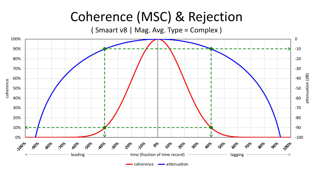
However, in order for a signal copy to have little or no effect on the frequency response of the direct signal, it suffices for its relative level to be down by 10 dB or more (isolation) which already happens once it’s leading or lagging by a mere 40 percent or more of the time record duration, even though the time analysis window is still ajar and not fully closed.

This leaves us with an important milestone. When misalignment, that biases coherence, within the time analysis window is the only known cause for coherence‑loss, 40 percent or more time offset corresponds with an amplitude reduction of 10 dB or more.

Judging by the fourth row of the table in Figure 1, this condition is already met for frequencies above 1.25 kHz after 16 milliseconds (or 5.5 meters). Let’s see how we can put this to use in the following example.

Claustrophobic

Figure 3 shows a section view of small venue were a single point source covers the audience. In such close confinements, depending on the composition of surrounding boundaries, specular reflections are known to cause trouble.

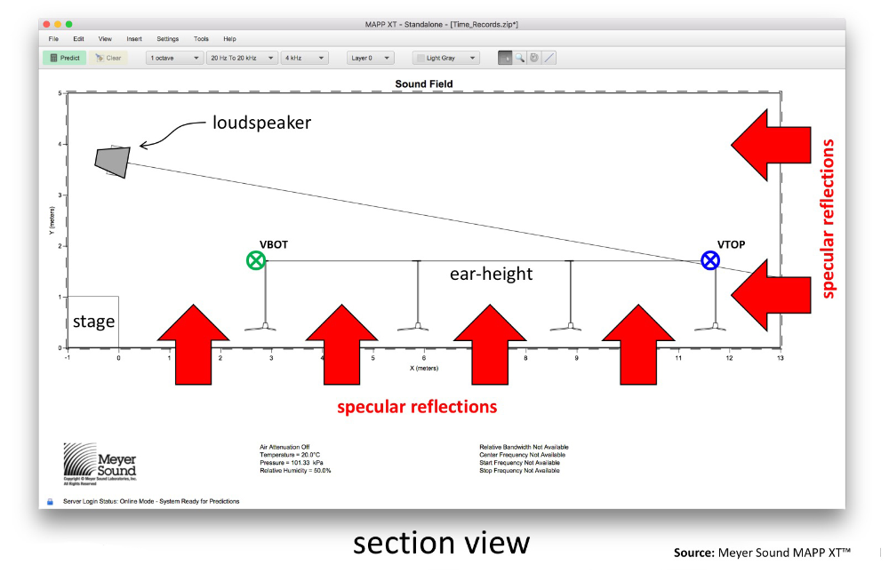
When we focus on the effects of a single boundary, e.g., the floor, we can exploit the “waterhouse‑effect” and use mirror images to mimic the reflections expected to originate off the floor.

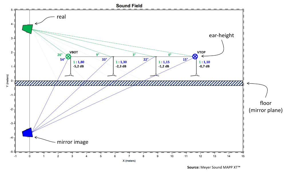
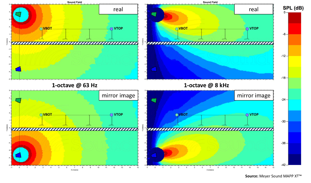
Figure 4 demonstrates the corresponding approach, and in prediction software we have the luxury of looking only at the direct sound, reflected sound or both. Let’s look at the results first and compare the sum of both direct and indirect sound to only the direct sound, at each of the four microphone positions.

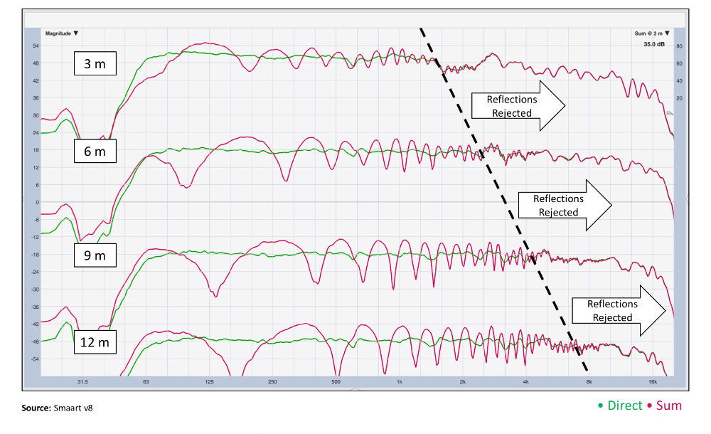
Notice in Figure 5 that depending on our distance, certain higher frequencies are functionally free from reflections, showing no signs of comb filtering, with little or no smoothing applied. In order to better understand why this is, we need to peel the onion.

Disclaimer: Ground‑plane measurements short‑circuit the “floor bounce” all together, by turning your measurement microphone effectively into a boundary microphone. However, you might find yourself outside of high-frequency coverage or measure the loudspeaker that’s intended for someone else at ear-height (line arrays) or the high frequencies might end up being occulted.

Layers Of Complexity

There are at least three layers of complexity to consider: 1) range ratios (relative level); 2) angular attenuation (relative level); and 3) time offsets (coherence).

At ear-height, the real loudspeaker is, at all times, physically closer than its mirror image and therefore louder (inverse square law) independent of our distance to the stage (Figure 4). At ear-height we’re always more on‑axis to the real loudspeaker than to its mirror image (again, Figure 4). For those frequencies, in the custody of the horn, where the loudspeaker responds to physical aiming (angular attenuation), it’s therefore louder, independent of our distance to the stage (Figure 6).

At ear-height, the real loudspeaker is always leading with respect to its mirror image. While the mirror image loudspeaker’s lag is expected to be some constant value for each microphone position, it will represent a different fraction of each of the multiple time records, affecting both coherence and attenuation proportionally, provided you use vector (complex) averaging.

Figure 7 depicts the individual measurements for the most distant microphone position at 12 meters. The top magnitude plot shows the sum of both direct and indirect with vector (complex) averaging. The bottom magnitude plot offers direct (real loudspeaker), indirect without windowing (mirror image loudspeaker), and indirect with windowing (mirror image loudspeaker). Coherence in the bottom pane belongs to the indirect sound, regardless of whether windowing is applied or not.

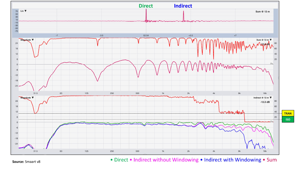
This far into the room, the range ratio is functionally 1:1 (once again, Figure 4), so little or no help from the inverse square law is to be expected. There’s also little or no angular attenuation (separation) as you can tell from the pink trace which is the response of the mirror image loudspeaker pre‑windowing (you get this result using RMS or polar averaging). Figure 6 confirms this for 8 kHz, where we see only one color division (3 dB for the most distant microphone.

It’s not until we apply vector (complex) averaging that the indirect sound is further attenuated because it’s late with respect to the direct sound. Above 10 kHz, we’re now functionally isolated from the floor “bounce” because its coherence is less than 10 percent.

One microphone position closer, at 9 meters (Figure 8), the direct sound gains market share because the real loudspeaker is closer, more on axis, and its mirror image is late by a bigger time offset than at the previous position.

For each microphone we move closer, this trend continues, and the joint effort of inverse square law, angular attenuation and coherence have rendered the upper half of the audible spectrum free from artifacts. I hope by now you can appreciate the extra rejection that can be achieved with help of vector (complex) averaging.

Never In The Last Row

It’s for this reason that you will never see me measure at the last row, in front of a specular wall. I always measure at the second‑to‑last row, where I intercept the sound destined for the last row (Figure 9).

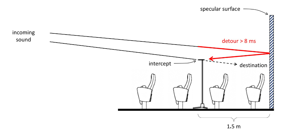
At 1.5 meters in front of the rear wall, the sound will be negligibly louder, but whatever sound is reflected of the rear wall will be late by 8 ms or more and not show up in my measurement for those mission‑critical frequencies (Figure 10).

Knowing your time records increases your confidence in interpreting the data and pick the battles you can win. It allows you to strategically position your microphone in order to get actionable data without having to resort to ill‑advised additional windowing or excessive smoothing, which set the table for poor EQ choices.