Impulse Response and Frequency Response. The impulse response of a device – an analog filter, a digital filter, a loudspeaker or even a room – is the reaction or response of the device over time in response to an input pulse.
Theoretically we can put a voltage, digital or acoustic pulse into a loudspeaker, amplifier, processor or room and record the output voltage, digital signal or microphone waveform over time to obtain the impulse response. However, a pulse doesn’t have enough energy at all frequencies to excite a device with enough level to give a reasonably clean signal above ambient noise (or a signal-to-noise ratio – SNR) at all frequencies.
Today many measurement systems use either a sinusoidal sweep or cyclic pink noise. (Dual FFT methods use any audio signal – like the output of a live mixing console – but that’s another story.) Sweeps and cyclic pink noise signals have enough energy at all frequencies to give reasonable SNR and therefore give a usable or stable impulse response.
The frequency response is the frequency-domain behavior of the device. It’s also the frequency-domain equivalent of the impulse response. (The term transfer function is sometimes used in place of the frequency response.) The frequency response is usually plotted as the magnitude (in dB) and phase (in degrees) across frequency. The frequency response can also be converted from magnitude and phase to a complex number representation; real and imaginary values for each frequency point.
Note that the time-domain impulse response and frequency-domain frequency response are inherently linked and are mathematically equivalent characterizations of the device. We can convert the impulse response to the frequency domain using the Discrete Fourier Transform (DFT) and convert the frequency response to the time domain using the Inverse Discrete Fourier Transform (IDFT); subject to some constraints that we won’t go into here. The fast implementations of these operations are called the Fast Fourier Transform (FFT) and the Inverse Fast Fourier Transform (IFFT).
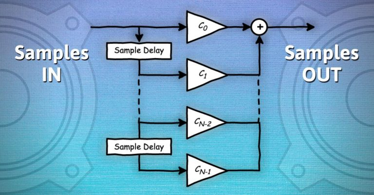
Returning to the “averaging” filter example: The impulse response of a digital filter is the output of the filter when we pass an impulse – a sample value of 1.0 – through the filter followed by zeros. Let’s calculate the impulse response using Figure 2.
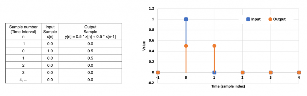
For this filter, the impulse response is [0.5 0.5] for the first two time intervals, and zero everywhere else. Its length is two samples, and since this length is finite, the filter is a finite impulse response or FIR filter.
Also, because this filter “averages” pairs of samples, we would expect large sample differences to be smoothed out, and very low sample changes to mostly be unaffected. Let’s look at the frequency response magnitude in Figure 3.
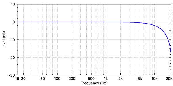
Sure enough, the averaging filter is a low-pass filter. Low frequencies, where the audio signal varies more slowly over time, are unaffected, but high frequencies are attenuated.
What happens if we change the sign of one of the coefficients in the averaging filter? A “difference” filter is created, as seen in Figure 4, and as an equation, we can express this as:
yn = 0.5 * xn + -0.5 * xn-1

This filter cancels out adjacent samples that are the same, or similar, and emphasizes pairs of samples that are very different. The difference filter’s frequency response is quite different to that of the averaging filter, which can be seen in Figure 5.

The difference filter is a high-pass filter. High frequencies are mostly unaffected, but low frequencies are attenuated.