Editor’s Note: This is part 1 of a 3-part series that can be accessed here.

The advantage of distributing subwoofers in front of the stage and improving the dispersion pattern of the configuration either by digital signal processing or physical setup is well known and used in many applications. The algorithms to calculate the delay values are usually implemented in the manufacturer’s software and are not accessible to the user. When using different programs, it can be seen that the calculated parameters for an identical array configuration vary between the different software solutions.

Since the theory of horizontal transducer arrays and their radiation behaviour have been analysed in detail in several publications, it seems interesting to know which approaches are commonly used to calculate the delay parameters, how they affect the directivity and which approach offers the best performance.

This series of articles gives an overview of the results of different algorithms, evaluates their performance in an independent simulation environment and compares the results with measurements on a physical array configuration. Part 1 )which you’re reading now) summarizes the results of a parametric study carried out with algorithms from different software to show the deviations between their approaches. Part 2 describes a comparison based on an objective metric to evaluate the performance of a simulated array configuration. A selection of parameters is used in a field test. The simulated and measured sound fields are analyzed in Part 3.

The frequency range of a subwoofer system is typically between 30 Hz and 100 Hz. Dedicated subwoofer systems sometimes operate below this range and main systems above it.

The radiation pattern of an array depends on the individual directivity of the single sound sources and the physical array configuration. Because of the wavelength in the frequency range of interest (11.32 m – 3.43 m) subwoofers are usually assumed to be omnidirectional. However, there are publications stating that this is not true for the entire subwoofer range (1). Besides the sound pressure increase, the arrangement of several elements in an array extends the acoustically relevant dimensions of the sound source and enables a higher directivity at low frequencies. The total length of the array determines the radiation pattern in the horizontal plane. Longer arrays have a higher directivity at the same frequency than shorter arrays. With increasing distance between the sources, the relative phase shift at a listening position increases, resulting in a destructive interference and inhomogeneous radiation behavior. To eliminate these effects, the elements should not be separated more than half the wavelength of the highest frequency reproduced by the array.

To meet the required sound pressure levels and spatial conditions, the radiation pattern may need to be optimized. Therefore, the relative time and level relationships between the sources can be adjusted. Greater delay on the outer elements increases the virtual displacement of the sources. This reduces the sound pressure level in the main radiation direction and widens the main lobe to achieve an expected dispersion pattern.

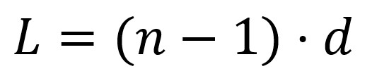
To get a feeling for how an approach of a delay algorithm can be designed, a parametric study was conducted to analyze the resulting delay values dt for a given set of input parameters. The input parameters are the number of elements n, the distance between the elements d or the resulting length L, and the nominal opening angle α. The following relationship exists between the mechanical configuration parameters:

Special attention is required if the mechanical configuration is influenced by the type of loudspeaker, e.g., with its dimensions the loudspeaker changes the mechanical configuration of the array thus influences dt. To create an appropriate test environment, the same conditions should be used in each software.

During the tests it was observed that the software (SW) offer different options for setting the environmental conditions, e.g., the temperature or the speed of sound c₀. 343 m/s or a temperature of 20 degree Celsius was used for all tests. To reduce the influence of the loudspeaker model, 18-inch loudspeakers or a similar size were chosen for the analysis, one loudspeaker for each position. However, most curving algorithms were found to be independent of the loudspeaker type.

Twenty-two (22) tests divided in three series were performed for six algorithms. In each series, only one parameter was changed at a time, namely the distance between the elements, the number of elements and the nominal opening angle. The tests included extreme values, such as α greater than 180°, very small distances between the elements or the behavior with even or odd numbers of loudspeakers. In addition to an analysis of the absolute delay values, the general delay strategy and software-specific features were studied.

Inter-Element Spacing

The distance between the elements determines the highest frequency that can be reproduced by the array without destructive interference in the main lobe. The relationship can be described by the wavelength:

In most software programs the multiplier k_λ is defined as 0.5, which equals half the wavelength of the higher cut-off frequency. However, two programs give a k_λ of 0.66. This leads to stronger sound pressure variations in the audience zone. To reduce comb filtering as much as possible, f_max refers to k_λ 0.5 in the context of this article.

For the first series of experiments, the nominal values α = 90° and n = 8 are kept constant. All algorithms calculate with constant distances between the elements. Figure 1 shows the normalized virtual position of the array elements over the delay values in milliseconds for a distance between the elements of 0.6 m and 2.5 m ( f_max = 286 Hz and 69 Hz respectively).

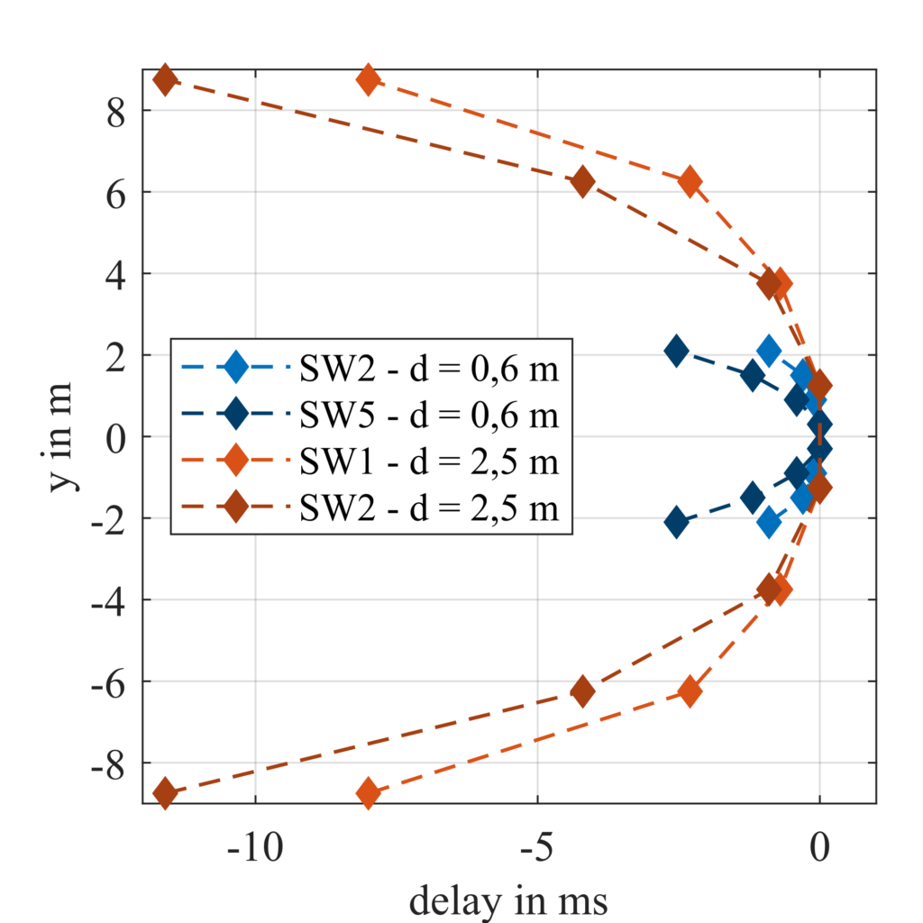
The diamonds describe the virtual position of the sound sources. Only the algorithms that provide the maximum and minimum delay values for the two tests are shown. With an element spacing of 0.6 m the differences are small, 1.9 ms for the maximum values of the outer elements. With an element spacing of 2.5 m the deviations increase drastically to 3.6 ms between SW1 and SW2. This corresponds to a physical path difference of 1.2 m and a phase shift of 130° at 100 Hz.

Array Length

The length of the array can be varied by adding more elements, while d = 1.05 m ( f_max = 163 Hz) and α = 90° remains constant. Here, a special feature of SW2 becomes clear. For small angles or short arrays this algorithm does not set delays, see Figure 2.

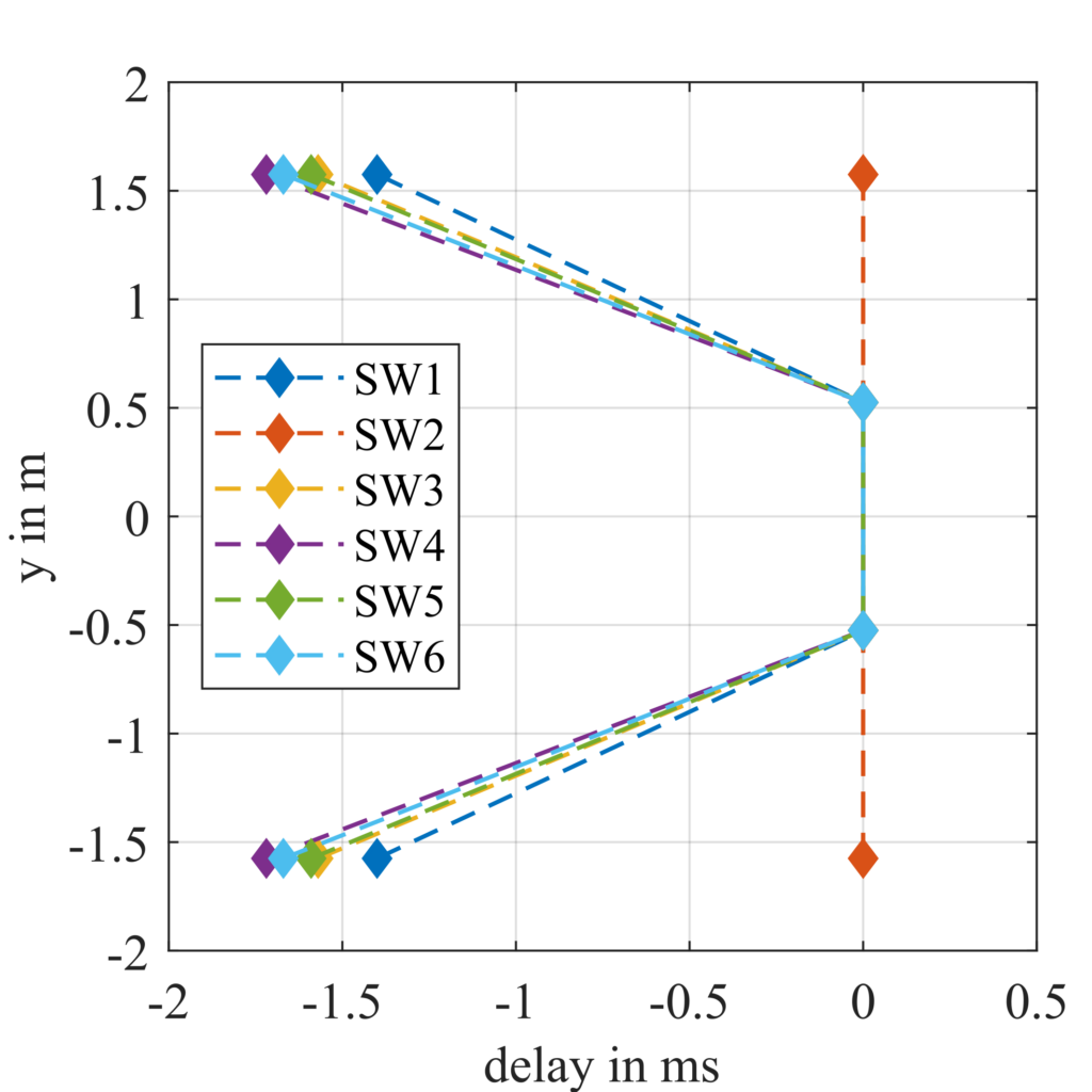
The algorithm defines a minimum coverage angle for the configuration depending on the array length. The longer the array, the smaller this nominal coverage angle. For the given example of L = 3.15 m, it was defined to be 93°. For opening angles α smaller than this coverage angle, no delay values are specified. The software does not provide any further information on this. Also, no mathematical relationship could be found that corresponds to the known array theory. With increasing array length, the differences between the delay values also increase in this test series.

Opening Angle

An analysis of the opening angle dependency is of particular importance for the tests. This value is used to optimise the radiation pattern for a specific audience zone. In this test series, the array consists of 12 elements that are 1.05 m apart. It can be seen in Figure 3 that the qualitative shapes diverge with increasing curvature.

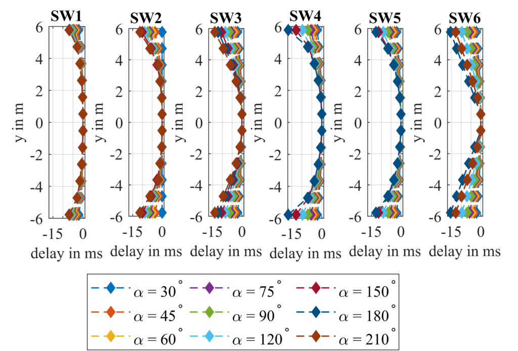
SW6 is the only algorithm that follows an almost linear increase towards the outer speakers. SW1 sets for all curving angles the smallest delay times. The increase to the outer elements is slower and more continuous compared to the other algorithms. This software and also SW6 do not allow opening angles larger than 180°. For larger opening angles, the difference to 180° is subtracted from the current parameter. The resulting delay values for α = 210° and α = 150° are the same. A comparable approach is taken for the algorithms of SW2, SW4 and SW5. However, they do not provide results above 180°. Only SW3 provides increasing delay values for opening angles of more than 180°. As already discussed, it can be observed that SW2 does not set any delay times below a minimal coverage angle. It is defined by 32° for this configuration. SW4 provides the longest delay times and therefore directs a lot of energy towards the sides. None of the software solutions uses gain tapering to influence the radiation characteristics of the array configuration.

Conclusion

Despite known analytical descriptions and complex models for array systems, a high deviation in the results can be observed. The same input parameters lead to significant quantitative differences in the delay times of the array elements. Furthermore, the optimization software show large differences in the qualitative curving approaches. From a pronounced, almost circular curvature behaviour of SW3 and SW4, a strong broadening of the main maximum is to be expected. With SW1, the user gets much shorter delay times that have a more elliptical profile. SW6 is the only algorithm that offers an almost linear increase in delay times.

The resulting sound fields and the performance of the different algorithms will be discussed in Part 2 of this series.

(1) Hill, A. J. (2018, August 30 – September 2). Practical considerations for subwoofer arrays and clusters in live sound reinforcement (Conference Paper). 3rd International Conference on Sound Reinforcement, Struer.