
Modifying the directivity characteristics of loudspeaker arrays through electronic delay has become increasingly popular.
Whereas 20 years ago the only option was expensive dedicated digital delay units, and a few years later the original BSS Omnidrive was a luxury, the advent of inexpensive digital processing has changed the game.
The design of complex arrays using a relatively high number of processing channels, as required to electronically modify the directionality of an array, is now affordable and widely implemented.
However, virtual (electronic) modification of an array’s directivity is not always a substitute for good old mechanical arranging or aiming, as the two methods have widely differing radiation characteristics off-axis (i.e., to the back and sides).
Let’s look at the differences in the two approaches, how they differ across a number of array types, and suggest applications where each of them should be used with subwoofers.
Arrival Times
The reason why physically moving a loudspeaker backward is different from delaying it electronically may not be intuitively obvious, but is easily shown graphically.
Figure 1a shows two loudspeakers (“A” and “B”) located left and right at equal distance from both a listener positioned in front and another listener positioned behind.

Leaving aside subtleties such as the location of the time origin of the loudspeakers, since it does not influence the basic concept being discussed here, sound from loudspeakers A and B will arrive at the same time to both listeners.
If we move back loudspeaker B (Figure 1b), then loudspeaker A is closer to the front listener, so sound reaches that listener earlier. Behind the loudspeakers, of course, the opposite occurs.
If we return the loudspeakers back to their original positions, and then apply electronic delay to loudspeaker B (shown in Figure 1c as a diverted path length to the listeners), we see that the output of loudspeaker A arrives earlier than B in both cases (in front and behind).
Thus, it is graphically clear that physically moving enclosure B produces a significantly different result to electronically delaying it.
Focus On The Effect
Let’s now look at the implications within the context of a vertical array of loudspeakers, and predict the coverage of a column of omnidirectional sources.

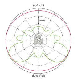
I often prefer to display results via polar plots, because with plane mappings it’s often difficult to understand the behavior at distances other than those close to the system being modeled.
Also note that I’ll use mostly omnidirectional sources instead of “real-world” sources (with a certain degree of attenuation at the back, i.e., not perfectly omnidirectional) to focus on the effect that the arrangement is causing on the directional response of a single loudspeaker.
In Figure 2a and 2b, we have physically tilted a 12-element array that is 23 feet (7 meters) long downward by 30 degrees.