The frequency axis of Figure 1 is marked at third-octave intervals. Note the improved selectivity of the raised cosine filter; it provides more precise third-octave selectivity, whereas the parametric filter leaks into neighboring third-octave bands.
A closer look at this figure shows that the parametric section leaks into more than three neighboring third-octave bands. The raised cosine filter doesn’t leak into other bands at all.
The Contour’s raised cosine filters give you surgical precision to adjust a frequency response.
The raised cosine filter not only provides improved selectivity, it also allows for perfect summation between neighboring filters.
This ability results in a significant advancement in graphic equalizer technology.
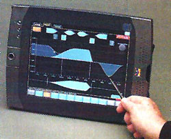
Figure 2 shows a portion of the third-octave graphic equalizer interface provided by the Contour Controller software.
The neighboring filters sum flat and third-octave selectivity is precise among the filters.

TRADITIONAL VS. CONTOUR EQUALIZATION
A graphic equalizer is comprised of a fractional octave filter bank. In professional applications, third-octave graphic equalizers are typical. To cover the audio spectrum, 32 third-octave bands are usually provided, from 25 Hz to 20 kHz.
Due to the implementation of these traditional filters, they interact with each other. The sides, or “skirts,” of these filters interfere with the neighboring filter bands. This interaction results in non-intuitive frequency responses, since the graphic equalizer controls do not reflect the actual response of the filter bank.
For example, let’s compare some different EQ shapes on a conventional graphic equalizer with the Contour equalizer. We pulled up seven faders on a graphic EQ, to boost a region from 500 Hz to 2 kHz by 6 dB, and then did the same in the Contour Controller software. See Figure 3 for a comparison of the results of the measured responses of these two equalizers. The transfer function of both devices was measured, and the resulting traces show the differences.

As you can see, Contour’s measured response shows a perfectly flat 6 dB boost from 500 Hz to 2 kHz. The traditional graphic EQ’s response is not what we expected. Because of the interaction between the filters, the overall boost is much higher than 6 dB, at some points the response reaches 10 dB of boost. There isn’t a single point in the graphic EQ’s response that is at the desired level of 6 dB. The graphic EQ’s “skirts” leak for more than an octave in both directions as well.
Let’s look at another example. Pull one filter up by 6 dB and another down by 6 dB. We did this a few times to see what happens when neighboring filters provide boost and cut functions. And again, we measured both devices to compare their responses, shown in Figure 4.

Contour’s response is exactly what we expected, 6 dB boosts and cuts at the desired frequencies. In the graphic EQ, due to the interaction between the filters, the boosts and cuts never get to 6 dB. For the final comparison, we tried to make a gentle transition across a few third-octave bands. Starting with a 2 dB boost, we then increased the boost to 4 dB and then 6 dB, coming back down the other side 4 dB and then 2 dB. We then did the same with Contour and then measured both devices, with results in Figure 5.

The Contour’s trace matches the desired response exactly, whereas the graphic EQ does not. Again, the graphic EQ’s response provides too much boost. The graphic EQ’s function leaks for over an octave in both directions. The bottom line is that with Contour EQ, neighboring filters do not interact in the traditional way.