As technology marches on, FIR (Finite Impulse Response) loudspeaker presets are becoming increasingly common, and with good reason – they’re not just a marketing buzzword. FIR filters offer some real benefits in pro audio applications, and, like any other tool, they come with their own drawbacks and considerations.

I’m often asked how FIR filtering works. For a more technically rigorous explanation, I highly recommend this article from Eclipse Audio, developer of the excellent FIR Creator software.

Here, however, we’ll avoid plunging into the math and instead keep to the conceptual shores. Those familiar with the under-the-hood mathematics will pardon the broad-strokes explanation I’ll be presenting. For a look at how manufacturers leverage the benefits of FIR for loudspeaker design, check out an interview earlier this year with my friend Sam Feine.

We start with a very important, foundational principle: time and frequency are inextricably linked. Mathematically, T = 1/f. T represents period, the time it takes for a wave to complete one cycle. f represents frequency, or the number of cycles per second.

This formula tells us that these two quantities are, mathematically speaking, two sides of the same coin. Different frequencies take different lengths of time to go through a cycle. So, we could say “Hey, let’s talk about that signal that cycles 200 times per second.” That’s 200 Hz. We could also say, “Hey, let’s talk about that signal that takes 5 milliseconds to complete a cycle.” That’s also 200 Hz. We’re just describing it in a different but equally valid way.

There’s a set of mathematical operations called transforms that take in time-domain data (a waveform) and spit out frequency-domain data (spectral analysis), or the other way around. This is how a spectrum analyzer works – even the basic RTA app on your phone – it looks at the audio signal picked up by the microphone (level varying over time) and transforms that into the frequency domain, displaying the frequency content of that signal.

So, let’s say we design a device that changes the level of different frequencies in an audio signal, or in other words, a frequency-dependent level control – better known as a filter. Perhaps our filter boosts the bass and reduces the highs.

By changing the frequency content of the signal, we are also affecting the signal in the time domain. It’s a mathematical certainty. (Example: grab Pre- and Post-EQ recordings of the same signal passing through your console. The difference in frequency content will be manifested in the two recordings having different waveforms as well.) This equivalence gives us a lot of flexibility and lets us do helpful and sometimes non-intuitive things in audio.

Everybody Clap Your Hands

Think about being in a reverberant space like a church. Let’s say we want to evaluate or describe the acoustic properties of the space. You could go into the space and fire a gun, pop a balloon, or clap your hands (for many of us who work in live sound reinforcement, walking into a venue and clapping our hands to evaluate the reverberance is a matter of habit). This sends out a wave of energy (we call it an impulse to illustrate the fact that it’s a very brief, very loud signal), and then we can record the energy as it came back from bouncing off the walls, etc.

Guns and hands and balloons are physical devices so there are limitations, but let’s assume for the sake of argument that the impulse we produce is incredibly loud for a very short amount of time and has a flat frequency response (contains all frequencies equally). So, you might imagine creating an audio file that has every sample value set to 0, except a single sample value at 1 (Full Scale). In fact, you can open an audio editing program and create such a file.

Figure 1 shows what it looks like when viewed in [Rational Acoustics] Smaart’s Impulse Response mode.
In the middle pane, time runs left to right on the horizontal axis and we can see that all the energy is concentrated around a single moment.

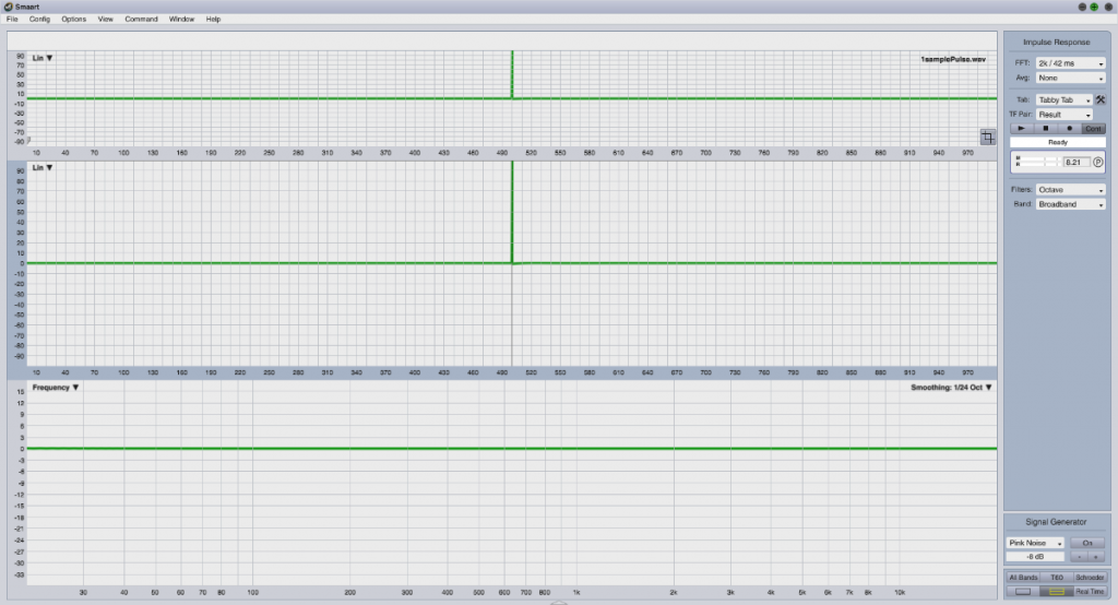
In the bottom pane we can see the flat frequency (more accurately, magnitude) response. Interestingly enough, those two statements are linked at the hip. If one is true, they both have to be true. If the energy were to be spread out over a longer time period then the magnitude response would no longer be flat from DC to light. Likewise, if the magnitude response is not flat from DC to light, the impulse cannot be infinitely short. Since our real-life devices are bandlimited to various extents, there’s no escaping this.

Why? Remember that we’re looking at the same audio file in both plots here – we’re just displaying the data in different ways. Put another way – if we change the frequency content of a signal, we change its waveform, and the converse is also true. If you’re stuck on this, check out my article “Clip To Be Square” here on ProSoundWeb that explores this concept in more detail.

Pull The Trigger

So – back to measuring the acoustic behavior of our hypothetical venue. Let’s create an impulse in the space (firing a starting pistol, clapping our hands, or popping a balloon are all reasonable approximations for our purposes here). We’ll set up a measurement microphone in the space and record the result.

As the energy bounces around the room and arrives back at the microphone, our recording will capture the level over time, and that tells us something about the space. Think echolocation or a Batman gadget. This is called an Impulse Response and it shows us the acoustic properties of the space. (Or, in the more general case, an impulse response is exactly what it sounds like: it describes a system’s output when an impulse is applied to the input.)

In the early days of studying room impulse responses, this data was recorded using a machine that trailed a pen over a scrolling roll of paper. Thanks to some cool mathematical tricks, modern audio analyzers can actually use a variety of different test signals (most commonly sweep tones and period-matched pink noise) to produce the same resulting IR data.

As a result, we don’t have to create the impulse sound in the space directly – the analyzer can produce the IR using other acquisition methods, which basically means the resulting impulse response file is “here’s the result you would get if you did play a pure impulse into this space.” If you play back the resulting IR (usually a .wav file), it sounds exactly like you might think: a snap or a pop with a reverb tail.

Acoustic measurement software can then analyze this impulse response data in multiple ways depending on what we’re trying to study. The top pane shows a linear view – this is level (vertical axis) over time (horizontal axis) and is basically the same thing you would see if you opened the IR file in a DAW or other audio editing software – viewing the waveform directly (Figure 2).

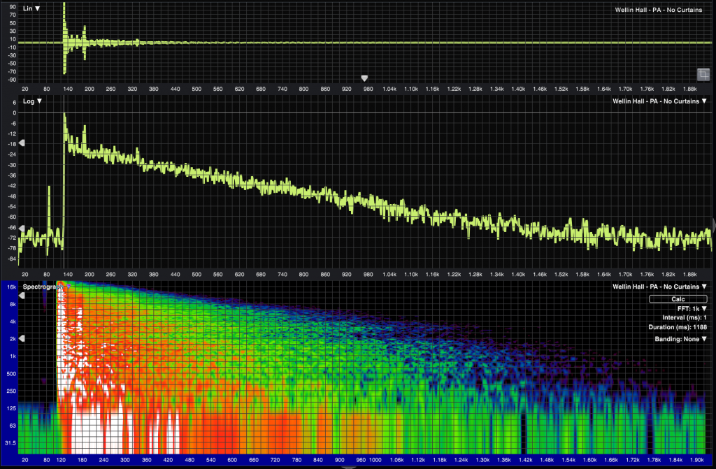
The middle pane is the same idea, only the vertical scale is in dB (logarithmic display) which makes low-level signal and decay behavior a lot easier to see. The bottom pane is a spectrogram rendering, with time moving left to right, frequency from low to high, and color representing level. We can see that this venue has longer reverberation at lower frequencies than at higher frequencies, which is pretty typical.

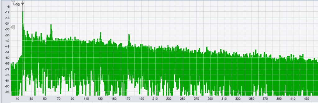
Now let’s look at a different room Impulse Response so I can point something out (Figure 3). Again, time runs left to right. You can see the initial impulse at around 18 ms, followed by three distinct secondary arrivals (the following peaks). Those are reflections off walls. (At this point, then, you may be wondering about the previous IR we looked at, above, and why it shows a peak before the main impulse. That “pre-arrival” is the result of using a swept tone test signal to measure a system that is exhibiting harmonic distortion – which is an interesting topic for another article.)

Now that we’ve captured the reverberant decay of the space, we can use it as a mixing tool. If we wanted to, we could get a good, clean, “dry” recording in our home recording studio, and then “multiply” that recording with the impulse response of the desired acoustic environment. Technically speaking, this process of multiplying a signal and an impulse response together is called convolution, and it’s how some reverb plugins work.

But for now, let’s revisit that first IR measurement we looked at – and swap the bottom spectrograph pane into a frequency response plot (Figure 4).

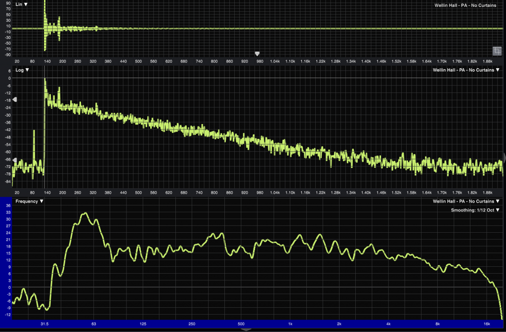
Here’s the key takeaway: these are both different views of the same data. Mathematically speaking, if you give us the impulse response of a room, filter, or system, we can generate the frequency response.

That goes the other way, too. We can take frequency response data and mathematically produce an impulse response that contains us the same information, just in a different format. We’re just transforming the data into a different format. (That’s the “transform” bit of fast Fourier transform.)

Let’s Talk About Tech

So now that we have a little more context, let’s talk about filters. Most of us are pretty familiar with EQ filters, so let’s think of those as an example. EQ filters are used to change the frequency response of an audio signal. Thanks to what we discussed above, we know that, since the filter has a frequency response, it also has an impulse response. If we have the frequency response of a filter, we know its impulse response as well (that’s the transform bit again).

Remember Figure 1 – the pure impulse with the flat frequency response – and let’s compare that to a filter. Figure 5 shows a bandpass filter (a filter that will pass energy in the midband and reject the low- and high-frequency components of a signal).

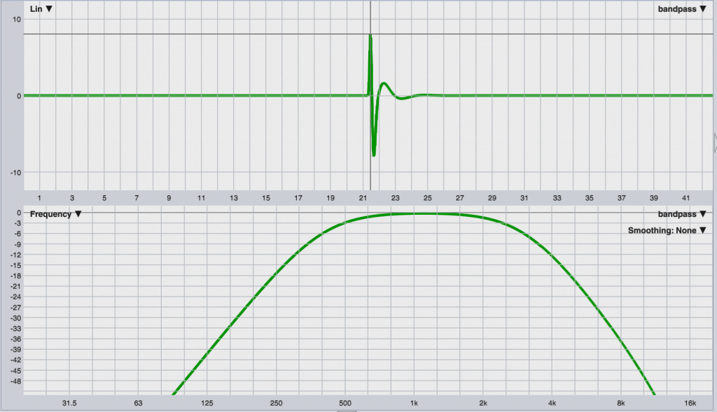
The bottom pane shows the frequency response of the bandpass filter – rolling off below 500 Hz and above 2 kHz – and the top pane shows the impulse response of that filter. Notice how the energy is no longer concentrated into a single clean peak. It can’t be, because we’re created a filter that treats energy differently at different frequencies, which means it treats energy differently in the time domain as well. That ripple and “time smear” in the IR isn’t a “side effect” of the filter’s response, it is the filter’s response – just viewed in the time domain.

Ones & Zeros

While we are used to thinking of the effects of filters in the frequency domain, an FIR filter can be thought of as the time-domain (impulse response) representation of the same response. An FIR filter is simply a list of numbers between -1 and 1 (“coefficients”). Each coefficient represents the output of the filter at that sample. 0 = no output here, 1 = max level output here. If we made a 9-tap (9-sample) filter of a perfect impulse (think about that .wav file we started off with), it could look like this: 10000000 – or – 000010000.

An FIR filter simply multiplies every single sample of the incoming audio signal by these filter values. Both of the examples would just reproduce the original input signal, with no change in level. They would behave differently in time: the first example has the impulse starting directly on the first sample, while the second one has it halfway through, producing four samples of delay.

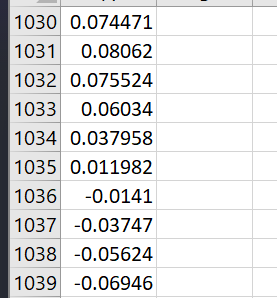
If you move from left to right along the filter’s IR and describe the magnitude at that point as a value between -1 and 1, that’s exactly what the FIR filter actually is. If you look directly at the sample values in a text editor, that’s what you’ll see (Figure 6).

So, conceptually, the FIR filter is based on creating the desired frequency response, then transforming that into the time domain to end up with a string of sample values that describe the impulse response. Then every sample in the incoming audio stream is multiplied (convolved) with these values, which produces the desired change in response to the signal. This is a mathematically demanding process, so FIR typically requires more computational resources than a more traditionally implemented IIR (Infinite Impulse Response) filter. So why should we use it?

First, we can create and implement a complex frequency response with a single filter, where creating the same curve with IIR filters might take a bunch of different parametric filters, shelves, etc., to combine into the target response. So, if you’re doing something like designing filters that will live inside loudspeakers to correct their response, a single FIR is much easier to get the results you need.

Second, we can create filters that affect magnitude and phase independently of each other if we want. Yes, they are inextricably linked, so it’s not magic. We pay the price in delay. That’s the difference between the two 9-tap impulse responses noted earlier. The one that doesn’t start its output until halfway through will take some more time to produce the output (because of that initial four-0 silence) but that delay allows us to manipulate the phase and magnitude independently within certain bounds.

If you look again at the FIR filter’s Impulse Response, notice that the peak is followed by a ringing/smearing of energy that makes up the filter’s response. Such is the nature of things – we can’t have a filter that creates output before it receives input – that would violate causality and probably explode the universe (if you figure out how to get this to work, call me and we’ll go to Vegas).

But we can have a filter that has a bit of delay (a bunch of 0-value samples) before the IR peak – and be able to implement filters that can manipulate magnitude and phase in a way that causes the IR to “smear” forward in time. For example, Figure 7 shows the same bandpass filter response from earlier, only with linear-phase.

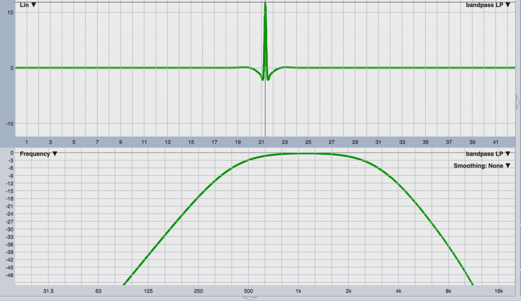
The magnitude response is the same, but the wiggles in the IR now extend in both directions – forward and backwards from the main peak. Because of this, the main peak arrival can’t be at the beginning of the filter’s value list – we have to push it back to allow room for some non-zero sample values before the peak happens. This is at the heart of why linear-phase FIR filters cause delay. It’s not “latency,” it’s part of the filter’s response before we get to the IR peak.

How much delay is required depends on the type of response we’re trying to implement, and what frequency ranges we want our filter to affect. In general, extending the filter’s response to lower frequencies requires more time (because T = 1/f). To dig deeper into this concept, see “FIR-ward Thinking” by Pat Brown on ProSoundWeb.

The Grand Compromise

But this is the practical limitation that prevents FIR from being more widely used in live sound applications. We need things to happen quickly. To affect lower frequencies with the filter, we have to remember that those frequencies take longer to happen (longer cycle time) and so we need to use longer and longer filters (more samples). That means more math, more system resources, and if we’re looking to go after phase separately, more delay through the filter.

The pro audio industry seems to have pretty much settled on a compromise where we are happy to tolerate a handful of milliseconds of delay in order to linearize the phase of our loudspeakers throughout the majority of the audible bandwidth – say, from 350 Hz on up – and below that point, we quickly get into diminishing returns, as every time we want to extend our filter resolution down an octave, we have to double the filter length.

As a closing example, Figure 8 shows the same linear-phase bandpass filter as before, with the bottom pane showing the Log view of the response, which better shows us the low-level details that aren’t visible in the Linear view. We can see that the filter’s IR occupies more than 15 milliseconds worth of time, and so we need an FIR filter that is long enough to accommodate that (and we typically also end up using something called a data window to “fade down” the tails to 0 towards the ends of the filter to avoid various undesirable effects).

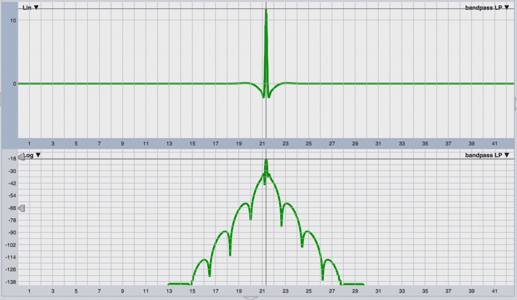
At 48 kHz, we might use a 1024-tap filter (1024 samples) which is 21.3 ms long, and since the IR peak is centered, will produce 512 samples (10.7 ms) of delay. That’s probably too much for a typical live sound application – but if we start to use shorter filter lengths, we’ll have to start truncating the “skirts” of the IR, which causes error in the frequency response.

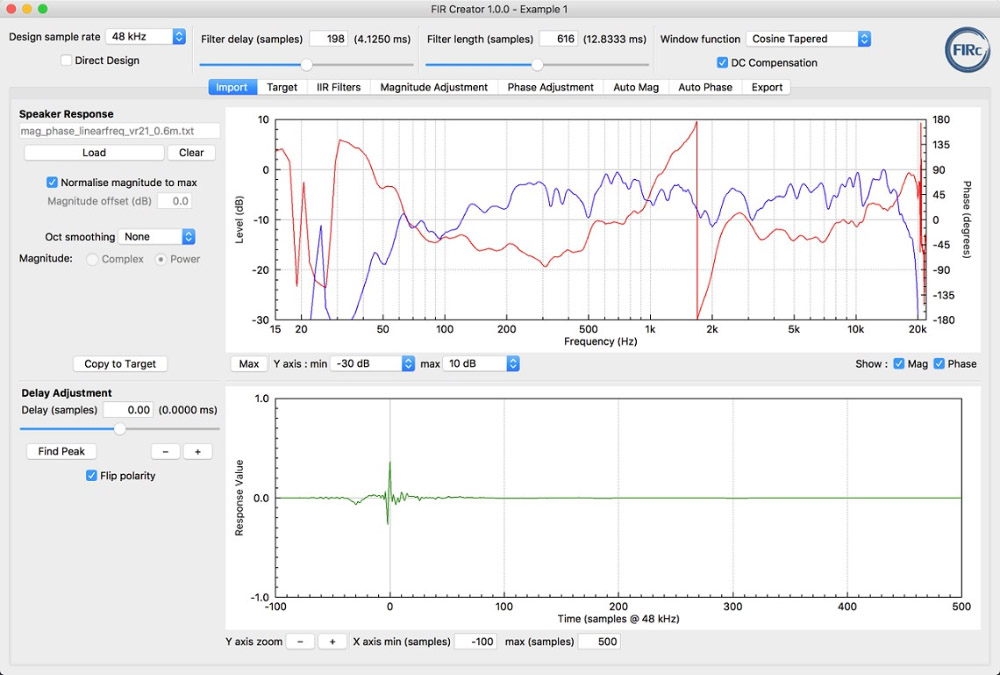
If you’d like to explore these concepts yourself, two common choices for generating custom FIR filters are FIR Creator from Eclipse Audio (eclipseaudio.com), which offers a free demo version, and FilterHose from HX Audio Lab (hxaudiolab.com), which offers a free LT version.