The wonderful silver lining of our present situation is that the internet is being flooded with all sorts of seminars, online classes, training videos, and the like. I’ve got a bunch of stuff bookmarked to dive into and it feels a bit like trying to drink from a firehouse.

However, I’ve stumbled across a few resources that seem to have some wires crossed regarding measurement theory and audio analyzers, so let’s take a minute and address some of the common mixups I’ve seen with regards to [Rational Acoustics] Smaart as well as other dual-channel FFT analyzers.

“FFT” Vs “RTA” Vs “TRANSFER FUNCTION”
Many resources conflate these terms. Here’s the scoop: FFT stands for Fast Fourier Transform, which is a mathematical operation that transforms time-domain data into frequency-domain data. In other words, FFT tells us what frequency components make up a signal.

Regardless of whether you’re taking an RTA or a Transfer Function measurement with an analyzer, the FFT is what’s happening under the hood to generate that data.

So trying to draw a comparison like “FFT vs RTA” is sort of like saying “Internal combustion engine vs Dodge Charger.” It makes a bit more sense to discuss RTA vs Transfer Function measurements, but both use FFT under the hood.

“FREQUENCY RESPONSE” Vs “MAGNITUDE RESPONSE”
The terms “magnitude response” and “frequency response” are often used interchangeably; however this is shorthand and it’s good to be clear on what we really mean for the sake of the folks who might not know the difference – kind of like that whole phase/polarity thing.

The magnitude response measurement displays magnitude over frequency, and the phase response measurement shows phase over frequency. The phase trace is a frequency-domain measurement as well, so in this context, the term “frequency response” collectively refers to both magnitude and phase over frequency. (Mathematicians use the term “Bode plot,” named for American engineer Hendrik Wade Bode, to describe this type of graph showing the frequency response of a system in magnitude and phase. Keep that one handy for the Sunday crossword.)

DATA WINDOW FUNCTIONS
Contrary to some claims, data window functions aren’t used to “fix rounding errors” or “infinitely repeating” decimal values. Here’s the deal: the textbook Fourier transform has a continuous frequency response running from 0 to infinity (DC to light, if you want to think of it that way).

However, in order for that to work, T = 1/f tells us that the input signal must also be infinitely long (or, in a more strictly mathematical sense, “continuous and aperiodic”). It’s not going to work too well for our purposes because we have sound check in an hour. So audio analyzers employ a Discrete Fourier Transform (DFT), which uses just a chunk of an input signal (which we call the Time Record or Time Window) and assumes that it’s infinitely repeating in a similar fashion. If you listen to a four-bar drum loop in your DAW, you know it will sound the same even if you loop it forever.

(“But wait,” you might think. “What’s all this “Discrete” nonsense? I thought they used Fast Fourier transforms.” The “Fast” bit is just a specific version of the DFT that can be calculated more efficiently, which is what allows us to carry out the analysis in real time. So FFT is just a special flavor of DFT.)

However, the whole “infinitely repeating” bit is an assumption that’s not true with real-world audio signals. If you’ve ever built loops in a DAW, you know the snap/crackle/pop nasties that are created by a bad loop edit. This causes a bunch of noise and error in the measurement that manifests by signal content at one frequency “bleeding” into the other frequency data points. Figure 1 shows how a 500 Hz sine wave spills over into the full spectrum of the measurement bandwidth.

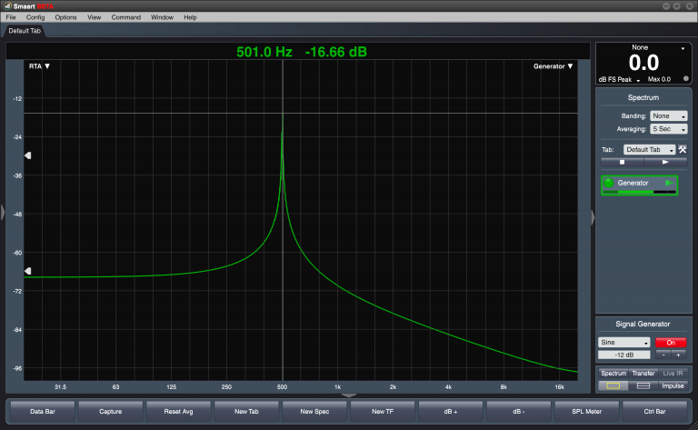
Enter the data window. If we “fade in” at the beginning out our selected signal chunk and “fade out” at the end, we’ve made the “infinitely repeating” assumption “more true,” because the end matches the beginning. That lets the DFT do its job with an input signal that matches its expectations. Figure 2 depicts the same measurement taken with a data window applied.

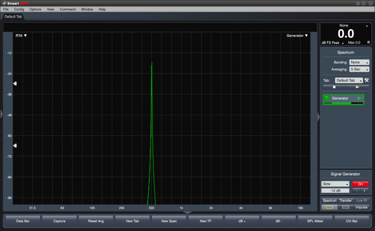
The spillage is greatly reduced, giving us a much cleaner measurement. There are a bunch of different data window options in most modern analyzers, but the default settings tend to be carefully chosen to give great results out of the box and shouldn’t require any tweaking in most situations.

TIME RECORD LENGTH & SAMPLING RATE
Sample rate is measured in samples/second (or Hz), and the size of data chunks used for each FFT operation is measured in samples, but these are two different concepts.

As with any digital device, the highest frequency that the analyzer can resolve is dictated by the sampling rate of your audio interface. In broad terms, HF cutoff (known as the Nyquist frequency) will be about half the sampling rate.

This concept should not be confused with the concept of FFT size, measured in samples. FFT size describes how many samples of data are used when calculating each frame of the measurement. Here’s the rule: In order to accurately describe a frequency via FFT, the data window must be open long enough for that frequency to complete a full cycle.

That’s it! It’s because the transform works something like this: For a 10 millisecond (ms) time record, the transform says “Hey, input data. Who went through one cycle in this chunk of time? You! 100 Hz! What’s your magnitude? What’s your phase? Cool. OK, next. Hey, who went through two cycles in this chunk of time? You! 200 Hz! What’s your magnitude? What’s your phase?” And so on. Data points (“bins”) fall at frequencies that make a full number of cycles within the time record.

A transfer function is commonly made by subtracting an electronic reference signal from an acoustic measurement signal. The measurement compares two signals and shows the relationship between them. We use the terms Measurement signal and Reference signal, but both signals can be pretty much anything we want. By the time our signals get into the analyzer, they’ve been converted to digital values, even if they were acoustic signals (sound waves) in a former life.

If you wanted to check that your two measurement microphones had matching responses, for example, you could place them nose to nose and take a transfer function measurement between them. This provides a comparative measurement between two mic output signals. Or maybe you want to measure the response created by an equalizer or system processor by taking a transfer function measurement between the input and the output of the device.

Once you realize that the analyzer will try to compare any two signals we feed it, you can see how a transfer function measurement can be used for a lot of applications besides measuring the response of a loudspeaker in a room.

LOOPBACK MEASUREMENT DELAY
In a common configuration, we configure the analyzer’s signal generator to output signal to two physical outputs on the audio interface. One is routed through the system we wish to measure, and the other is “looped back” to an input on the interface. In this way, we eliminate from the measurement any effects of interface latency.

The remaining time offset is a result of signal propagation through the system under test, not the latency of the computer-audio interface connection. In fact, that’s one of the reasons it’s not usually recommended to directly reference the internal signal generator – it keeps driver latency and interface latency in the picture, which can give some unexpected results.

COHERENCE TRACE
The coherence trace (not to be confused with the concept of phase coherence) functions more or less as a data quality indicator, serving to indicate the level of correlation between the measurement and reference signals. In other words, “How confident can we be that the energy showing up at the mic was caused by our reference signal?”

In order to avoid making decisions based on low-coherence data (the 60 Hz rumble caused by the HVAC or the subway under the theater should not be treated with EQ!), Smaart’s coherence blanking threshold hides data whose coherence values fall below the threshold. This is a display-only feature and has no effect on the underlying measurement data. It only controls whether or not those data points are visible on screen.