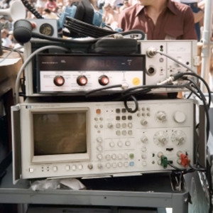
The display of the 3582 was four inches square, about the area of an iPhone, with only one color and 128 lines of resolution.
We could see one live trace and one stored trace at a time – both green! A grand total of two traces could be stored in its memory.
The modern analyzer shows amplitude and phase traces on separate screens. We did not have that luxury. The only way to see phase and amplitude together was to view their traces overlaid on top of each other.
This was such a bad idea that no other maker of analyzers has ever done it, but we were stuck with this method from 1984 to 1991.
It took 21 traces (seven linear frequency spans of amplitude, phase and coherence) to characterize a complete response at a single location. This means that we never had a complete record of the frequency response at any time. We would look at the lows, then work our way up through the mids and finally the highs. The process took about 1.5 minutes, so don’t complain to me about your analysis program being slow!
In addition, the lack of available memory traces made it difficult to remember what we had in the low end by the time we were looking at the high end. This state of affairs is difficult for the modern audio engineer to picture because we’re all now totally accustomed to a world of memory, presets and automation.
It was always interesting to see the reactions of engineers when they saw their first high-resolution responses. It’s like seeing a razor blade through an electron microscope, horribly ragged and disfigured, not at all like the smooth edge we see with our naked eye. Engineers had been accustomed to low-resolution, amplitude-only responses (the RTA). They knew there was much more going on than this simplistic view showed, but few were prepared for how bad a good system looks under a microscope. Oh, and a bad system? It just looks more bad than a good one.
Nonetheless, once one has viewed the high-resolution response, it’s impossible to ever look at an RTA the same again. You always knew there was so much that it wasn’t telling you, and now you knew that the answers were out there.
Phase
Every engineer had heard of phase response but almost none had ever seen one. We could see it in the first generation system (3582A), but it was broken into seven linear segments. It’s difficult enough to comprehend and decode a single span of phase data, but here we were trying to decipher seven segments into a composite response. It was like trying to paint a landscape while viewing it through a moving periscope.
Now try to explain this to the front of house and/or system engineer, who would look at the screen and conclude that the response was a pile of spaghetti. Seeing the phase response of a concert sound system in the room was a huge breakthrough, but only for a very small number of folks who could put the whole picture together. For the rest of us, phase would remain a mysterious, magical force.
Delay times had to be found by counting the number of wraparounds in the phase response for a given span of frequencies. For example, each wraparound would represent 1 ms of delay when we were measuring the 0 Hz to 1 kHz range, and 2 ms when we measured the 0 Hz to 500 Hz range.
We would know we had found the time correctly when we saw the phase flatten out horizontally on the screen. This was extremely difficult for several reasons.
The first is that reflections mixed in with the direct signal give the phase trace a modulated appearance, and it can be very challenging to discern direct from reflected arrivals. The second is that most loudspeakers at that time had phase responses that were highly variable over frequency. These loudspeakers were literally moving targets. We could find their arrival in the high end but then we were way out of sync in the mids and lows.
No loudspeaker has a perfectly flat phase response even today, but the models available in the early 1980s were orders of magnitude worse than the current models. Seeing phase in segments was a step forward from the RTA, which could not even calculate it. The extreme difficulty of reading the traces greatly limited the practical application of our new phase capability.
Coherence (Signal-To-Noise Ratio)
One of the standard features of the dual-channel FFT analyzer was coherence factor, which provides an indication of the analyzer’s confidence in the quality of its calculation. Coherence factor is derived statistically from averaged data. If every sample taken exactly matches, then the coherence factor is 1 (perfect stability). Conversely, if the samples are randomly related then the coherence is 0 (zero stability).
Any measurement we take of a device will contain some noise contamination. Coherence reveals the proportional strength of the noise contribution. A coherence factor of 50 percent indicates equal parts signal and noise. A loudspeaker measurement contains direct sound (on-time signal), reflected sound (late signal) and noise (uncorrelated signals like the HVAC system). The coherence factor is highest when the direct sound is strong and goes down as the late arrivals and noise gain strength.
Coherence is calculated at every frequency so it tells us which ranges are stable and which are struggling with noise. The practical benefit of coherence is that it helps to identify the causes of problems and therefore raises the probability of enacting the best solutions.