Quasi-Log Resolution
High-resolution analyzers existed in those days but were poorly suited for pro audio applications. The price for achieving high resolution was that the computations were linear in the frequency axis.
The fast Fourier transform (FFT) is derived from a time sample, unlike the parallel filter set of the streaming RTA. Time only comes in linear form as do the products of its computation. Linear frequency resolution is counter to our human perception, which is mostly log.
The win-win solution would be to put together a series of linear displays to build an overall log response, a linear/log hybrid. This provides the mathematical power of the FFT adapted to match the log tonal envelope of human perception.
It’s what is inside the modern analyzer even if you’ve never noticed it. However, you would certainly have noticed it in its first generation form, since the data came in a “some assembly required” kit.
The Early FFT Analyzer
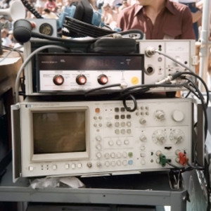
Meyer Sound began using the Hewlett Packard HP3582A dual-channel FFT analyzer for production testing and research in the early 1980s. This advanced tool was primarily targeted to research laboratories, industrial, military and institutional markets.
Our application at Meyer Sound was unusual for the 3582 to begin with, but then moved way out of the mainstream in 1984 when John Meyer and I began taking the analyzer out of the shop and into the concert halls. The 3582 needed lot of peripheral equipment to be able to measure and equalize in a concert setting. We’ll cover that after we explore the movement of the FFT analyzer into the mainstream.
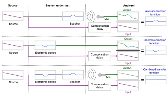
Figure 4: The three-pair transfer function measurement flow block (Room/EQ/Result). The acoustic, electronic or combined response can be found between the two measurement access points.
The 3582’s frequency response computation was created with 128 linearly spaced data points. This gave us 64 points for the upper-most octave, 32 points for the one below 16, 8 and so on. This is a tremendous amount of resolution for engineers accustomed to the 31 LEDs of the RTA. But once you see a high-resolution frequency response for the first time, you realize that a 1/3rd octave rendering is pretty much useless for our purposes.
Basically we had two to three octaves in clear view. We could never see the entire audible range at high resolution at the same time, but we could see all of it eventually by viewing the responses in series.
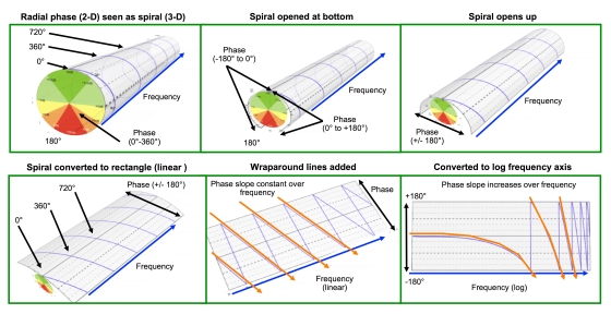
Figure 5: Phase response is “unwound” with displays in both the linear and quasi-log frequency axis. Note that the spacings are even in the linear display. (3-D artwork provided by Greg Linhares, courtesy of Meyer Sound)
Each linear response started at 0 Hz and then went up from there. The full-range response (0 Hz to 25 kHz, 5 ms time record) provided good resolution from 5 kHz and up. We had data points every 200 Hz, which was plenty in the HF range (10,000 Hz, 10,200 Hz, 10,400 Hz, etc.) but ridiculously low in the LF range. We could barely tell if the subwoofers were on or off with data points at 0 Hz, 200 Hz and 400 Hz!
We could get more LF resolution by reducing the range, i.e., not measuring all the way up the spectrum. The next range down (0 Hz to 10 kHz, 10 ms, 100 Hz resolution) gave us a good look between 2.5 kHz to 10 kHz. It went on like this in seven steps until we had a clear look at the low end (0 Hz to 250 Hz, 500 ms, 2 Hz resolution). We had 30 Hz, 32 Hz, 34 Hz in view so we had great LF detail, but could not see anything above 250 Hz. Yes, it was quasi-log: the analyzer handled the linear part, and your head handled the log part.