Talking About Resolution
The standard resolution for audio measurements in the heyday of the RTA was 1/3rd octave. This might seem sufficient at first glance but closer examination clearly reveals its limitations.
The answer lies in the “sampling theorem” which proves the need to oversample a particular parameter to ensure we have sufficient resolution to make decisions on that level.
For example, if we sampled the temperature every day at noon, we’d obtain a series of values and determine an average temperature. This would only be an accurate representation if the temperature never changed during the day or invariably got cooler at night.
We would obtain a very different average if we oversampled to twice a day by including midnight. Accuracy would be better yet if we measured hourly, and so on. Simply put, oversampling improves accuracy and leads to a better characterization of an infinitely divisible value. At some point we have to deem it sufficiently accurate to make conclusions.
The characterization of peaks and dips in a loudspeaker’s frequency response is also infinitely divisible. How fine do we need to slice it to make good decisions for sound system optimization? Is octave resolution enough? No way. We couldn’t differentiate a terrible response from a good one at that resolution. The most common finding for frequency response resolution of the human hearing system is around 1/6th octave, known as the “critical bandwidth.”
The RTA’s standard measurement resolution of 1/3rd octave leaves us vulnerable to peaks and dips that fall at the mid-points between the data center frequencies. This essentially gives us enough data to accurately set filters with a bandwidth of an octave or more, which is a very gross level of EQ action.
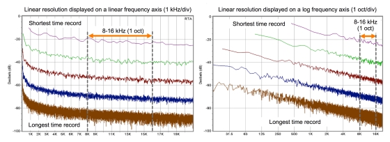
Figure 2: Linear vs. log frequency resolution: A single FFT response computes the data with linear frequency spacing, displayed here with both linear and log frequency scaling. The linear/linear display (left) shows equal spacing between frequency bins. The linear/log-spaced version shows wide LF spacing and progressively smaller spacing with frequency. Linear frequency resolution depends upon time record length, shown here in sequential quadrupling. Note the poor LF resolution (short time record) and the excessive HF resolution (longest time record). (Courtesy of Rational Acoustics Smaart).
Alas, the inherent errors of this system were not well known, and the most popular analyzer and equalizer pairing was one that had a matched set of sampling error blind spots: the 1/3rd octave RTA and the 1/3rd octave graphic EQ. Sometimes we get lucky and a peak in the system falls right on the center frequency of the analyzer and the equalizer. In that case we’re golden. Peaks that fall between the 1/3rd octave centers would first be inaccurately measured and then inaccurately treated with filters. Such a game of chance is not very attractive when our reputation is on the line.
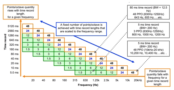
Figure 3: The fixed points/octave (PPO), also known as “quasi-log” or the Constant Q transform.