As explained on the previous page, the in-phase additions and the out-of-phase cancellations result in the peaks and valleys in magnitude frequency response respectively. The magnitude of these peaks and valleys can also be computed.
The feedback gain margin was set to 6 dB which means that the open loop gain was -6 dB and is equivalent to 0.5 in ratio. This can be obtained by using the anti-log formula as follows:
Ratio = 10^(dB/20) (Equation 3)
In addition to the original input of 1.0, an open loop gain of 0.5 means that each feedback loop is feeding half the amount of output back to the input. As discussed in Part 1 of this article, this corresponds to a series of numbers as follows: 1.0, 0.5, 0.25, 0.125, 0.0625, 0.03125 …..
Since the closed loop gain of the system is at unity, the eventual total magnitude at the output will be the sum of the above series of numbers. Since these numbers are in geometric progression sequence, the sum to infinity is given mathematically by the following equation:
Sum of series = 1/(1-r) where r is the open loop gain in ratio and for -1< r < 1 (Equation 4)
To calculate the magnitude of the peak in this example, we set r = 0.5. Therefore the peak magnitude is 1/(1-0.5) = 2. In decibel, this can be worked out by using the 20 log formula as follows:
Decibel = 20 x log(ratio) (Equation 5)
Using the above equation, the peak magnitudes are calculated to be 20 x log(2) = 6 dB.
To calculate the magnitude of the valley, each subsequent feedback loop is maximizing the partial cancellation from its previous loop i.e. will have the sign different from its previous loop. This results in alternating signs for the series of numbers as follows: 1.0, -0.5, 0.25, -0.125, 0.0625, -0.03125 …..
In this case, the r in Equation 4 has a value of -0.5. Hence, the sum of the series = 1/(1+0.5) = 0.6667. In decibel, the valley magnitudes are computed to be -3.5 dB.
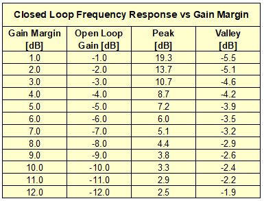
The calculated peaks of 6 dB and the valley of -3.5 dB correspond very well with the measured closed loop frequency response of Figure 19.
Using the above equations, the peaks and valleys at various feedback gain margins can be conveniently calculated in an Excel spread sheet as shown in Figure 20.
Another Example
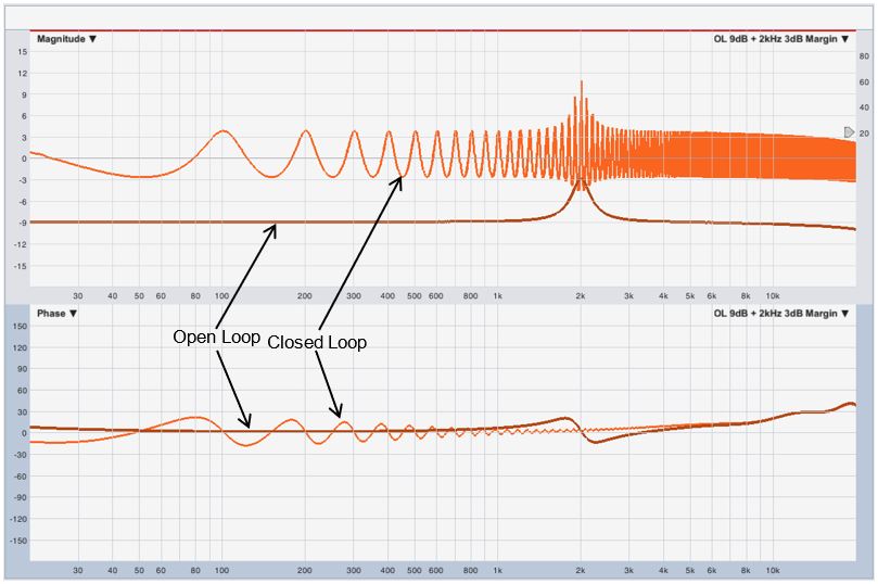
Using the same setup, closed loop responses of various open loop characteristics can be studied. Another example of the closed loop response with a 2 kHz peak in the open loop is shown in Figure 21.
Notice that in Figure 21, the 2 kHz peak in the open loop response has a low feedback gain margin of 3 dB and this has resulted in significant peak in the closed loop response. As shown in the table of Figure 20, operating at low feedback gain margin is not a good idea and will result in significant perturbations to the steady state closed loop frequency response.
Transient Response
To characterize the transient response of the closed loop system, continuous pink noise with a sudden cut off was used to feed the input. The time waveform was then analyzed for any added signal after the pink noise signal was terminated at the system input.
Figure 22 shows the waveform in the case where there is no feedback. This is accomplished by muting the mixer input channel for the feedback path. The red time cursor indicates the time corresponding to the sudden termination of the pink noise.
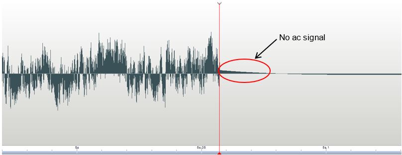
In the case of no feedback, pink noise at the system output terminated cleanly immediately after the red time cursor. The slight droop in the output time waveform after the red cursor was caused by the lower frequency limit of the system and the recording device. This is a normal manifestation when the system is not capable of responding to DC i.e. 0 Hz.
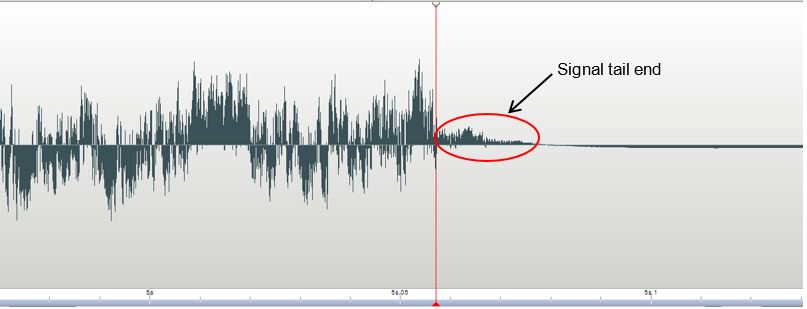
Figure 23 shows the time waveform of the case with the same open loop characteristics as Figure 21. In this case, there is considerable tail end signal at the system output after the pink noise at the input was terminated. This means that for a system with a delayed feedback loop, when the input signal ceases, the output will continue to pump out signal while flushing out the left over signal still existing in the feedback loop. This phenomenon is most clearly manifested when there is a sudden cut-off in the input signal.
Summary
In live sound application, there is unavoidable signal feeding back from the loudspeaker to the microphone. As long as the microphone can “hear” the loudspeaker, the contaminated signal is colored by the axis frequency response of the loudspeaker and that of the microphone; delayed by the path distance between the loudspeaker and the microphone; and its magnitude is defined by the open loop gain.
This unwanted signal will then be continuously added to the system. If there is insufficient acoustic feedback gain margin, this can result in significant magnitude variation in the system steady state frequency response as well as significant tail end in the system transient response. Significant efforts in achieving the smooth targeted loudspeaker system frequency response can therefore be easily negated with insufficient acoustic feedback gain margin in actual application.
In studio recording, headphones can be used for monitoring instead of loudspeakers to prevent unwanted sound from leaking into the recordings. In contrast, for live sound application where loudspeakers are inherent in the sound reinforcement system, sufficient acoustic feedback gain margin should therefore be adopted whenever viable to achieve the best possible reinforced sound quality.
In summary for live sound application, there will be trade-off between what is the affordable gain for the particular microphone channel which is characterized by the acoustic feedback gain margin and the closed loop system steady-state and transient performance.
You can also read Part 1 and Part 2 of this series.