Part 1 of this article explained the importance of the open loop function and how it can be examined to determine if the system goes into oscillation when the loop is closed.

The vectorial approach to compute the summation of two sinusoidal signals of the same frequency was also discussed. These concepts provide a good foundation for the following topic where the practical measurement of the open loop function is conducted.

Choosing Where to Open the Loop

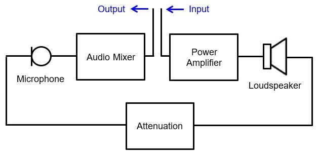
In Figure 4 of Part 1 of this article, it is impractical to inject the signal and measure the output of the open loop function since the parameter involved is sound pressure level.

However, the loop can be opened up at any point for open loop function measurement. A more convenient point to open up the loop is just after the audio mixer as shown in Figure 8.

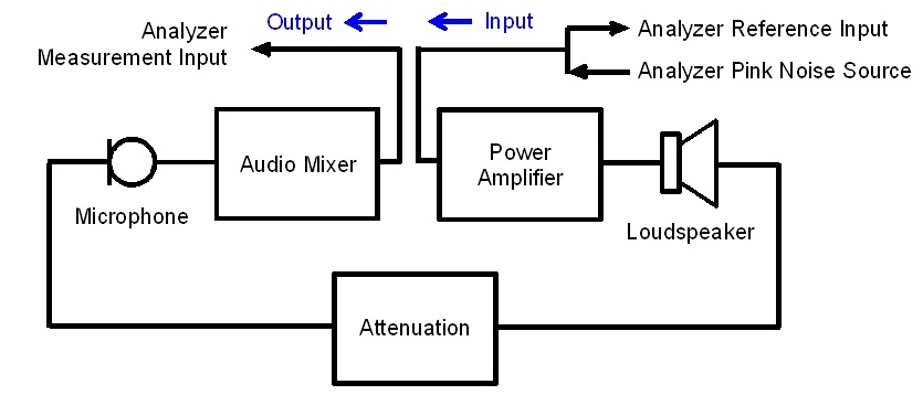
Since the loop is open up where the signal parameter involved is voltage, test signal such as pink noise can now be easily injected into the input of the open loop and the output response of the open loop can then be measured. Using a dual channel FFT acoustic measurement tool such as SmaartLive, the test set up connection is shown in Figure 9.

For a practical measurement of the open loop function, a graphical layout of the test setup with the associated signal flow diagram is shown in Figure 10.

In this test setup, the microphone is facing away from loudspeaker similar to a stage monitor application. Initially, there is no high pass filter or channel equalization for the microphone channel. The mixer output has some equalization just to obtain a reasonably flat on-axis response from the loudspeaker.

In Figure 10, there is a switch for selection between measurement mode and normal operation closed loop mode. For closed loop operation, the switch is initially toggled to Position 1.

To minimize the open loop gain measurement error caused by the input impedance loading by the audio interface, high input impedance on the audio interface inputs were used.

Since the absolute magnitude of the open loop gain is important, it is necessary to ensure that both reference channel and measurement channel of the audio interface device were calibrated. This was easily accomplished by feeding both of these channels with the same pink noise generator source via a Y-cable. The magnitude frequency response showed a flat trace and the audio interface device input gains were adjusted for this flat trace to line up at 0 dB.

To measure the frequency response plot of the open loop function of Figure 9 setup, the switch in Figure 10 was toggled to Position 2 and SmaartLive transfer function mode was used. The transfer function mode plots the magnitude and phase response of the ratio of the measurement input signal voltage to the reference input signal voltage. This was exactly what was required to obtain the open loop function. A sample plot of the magnitude and phase response of the open loop function together with the earlier calibrated 0 dB line is shown in Figure 11.

The top trace is the magnitude response and the bottom trace is the phase response. To avoid reducing the peaks displayed in the magnitude plot, no magnitude smoothing was used and that explains the spikey looking magnitude response plot. As for the phase response, phase smoothing was utilized for a more readable plot.

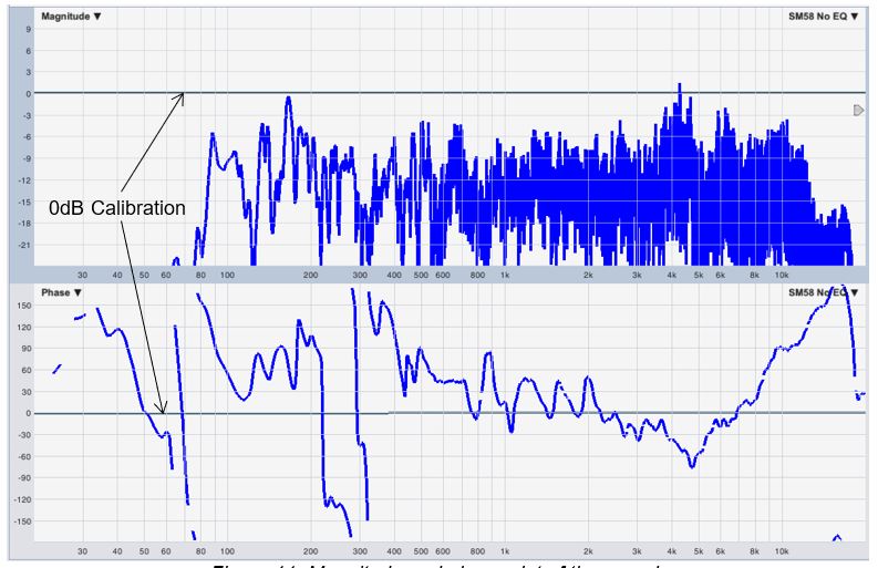
The dark grey line running across the 0 dB in the magnitude response and flat 0° line in the phase response is the calibration trace of the two inputs of the audio interface prior to the open loop measurement as described earlier.

The above magnitude and phase response plots were captured at a particular mixer channel fader level and without any channel equalization applied for the microphone. Since the mixer fader contributed directly to the overall open loop gain, pushing the fader up or down moved the entire magnitude frequency response plot up or down accordingly. As expected, the phase frequency response plot remained unaffected by the mixer fader adjustment.

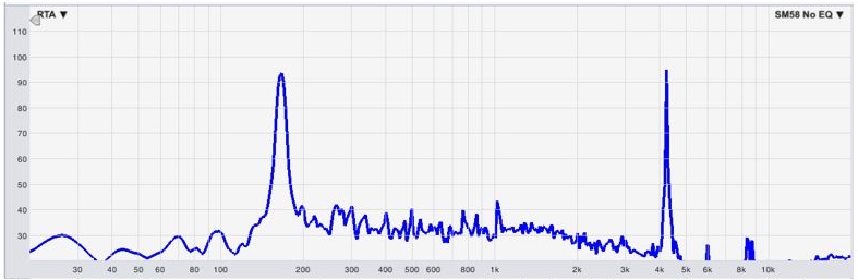
It is immediately observable on the magnitude plot that there are two high peaks, one at 166 Hz and the other at 4.25 kHz. Since the corresponding phases are not far from 0°, when the loop is closed, the resultant magnitudes of the output signal and the input signal would add up almost linearly. If the loop was closed (i.e. switch is toggled from Position 2 to Position 1 in Figure 10) at this setting, acoustic feedback might occur since the effective open loop gain approached unity to satisfy the condition for the system to just able to sustain a self-oscillation. When the loop was closed, the system did oscillate exactly at the two predicted frequencies as shown in the real time analyzer frequency spectrum plot in Figure 12.