

Some terms: The Fast Fourier Transform is an algorithm optimization of the DFT—Discrete Fourier Transform.
The “discrete” part just means that it’s an adaptation of the Fourier Transform, a continuous process for the analog world, to make it suitable for the sampled digital world. Most of the discussion here addresses the Fourier Transform and its adaptation to the DFT.
When it’s time for you to implement the transform in a program, you’ll use the FFT for efficiency. The results of the FFT are the same as with the DFT; the only difference is that the algorithm is optimized to remove redundant calculations. In general, the FFT can make these optimizations when the number of samples to be transformed is an exact power of two, for which it can eliminate many unnecessary operations.
Background
From Fourier we know that periodic waveforms can be modeled as the sum of harmonically-related sine waves. The Fourier Transform aims to decompose a cycle of an arbitrary waveform into its sine components; the Inverse Fourier Transform goes the other way—it converts a series of sine components into the resulting waveform. These are often referred to as the “forward” (time domain to frequency domain) and “inverse” (frequency domain to time domain) transforms.
For most people, the forward transform is the baffling part—it’s easy enough to comprehend the idea of the inverse transform (just generate the sine waves and add them). So, we’ll discuss the forward transform; however, it’s interesting to note that the inverse transform is identical to the forward transform (except for scaling, depending on the implementation). You can essentially run the transform twice to convert from one form to the other and back!
Probing For A Match
Let’s start with one cycle of a complex waveform. How do we find its component sine waves? (And how do we describe it in simple terms without mentioning terms like “orthogonality”? oops, we mentioned it.) We start with an interesting property of sine waves. If you multiply two sine waves together, the resulting wave’s average (mean) value is proportional to the sines’ amplitudes if the sines’ frequencies are identical, but zero for all other frequencies.
Take a look: To multiply two waves, simply multiply their values sample by sample to build the result. We’ll call the waveform we want to test the “target” and the sine wave we use to test it with the “probe”. Our probe is a sine wave, traveling between -1.0 and 1.0. Here’s what happens when our target and probe match:
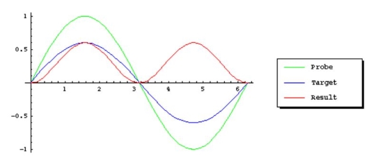
See that the result wave’s peak is the same as that of the target we are testing, and its average value is half that. Here’s what happens when they don’t match:
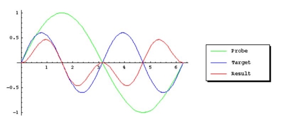
In the second example, the average of the result is zero, indicating no match.
The best part is that the target need not be a sine wave. If the probe matches a sine component in the target, the result’s average will be non-zero, and half the component’s amplitude.